Graphs
Graphs. The Graph ADT is useful in representing relations, such as prerequisite relations It’s quite commonly used for representing relations of adjacency or accessibility in a network. the network may be a communications or transportation network (of pipelines, roads, etc.).

Graphs
E N D
Presentation Transcript
Graphs • The Graph ADT is useful in representing relations, such as prerequisite relations • It’s quite commonly used for representing relations of adjacency or accessibility in a network. • the network may be a communications or transportation network (of pipelines, roads, etc.)
Applications of graphs • Typical graph-related problems are to determine • accessibility in a network, given adjacency info • whether removal of a node will disconnect a network • the cheapest path between nodes • whether a task is an indirect prerequisite of another
Graphs defined • A graph consists of • a set of vertices (or nodes) • and a set of edges (or arcs) • In a directed graph (or digraph), the edges go from one vertex (the source) to another (the destination). • In an undirected graph, the edges simply go between two vertices
Loops and multiple edges • A loop is an edge • from a vertex to itself in the directed case • between a vertex and itself in the undirected case • In either case, we usually disallow loops • We usually disallow multiple edges between the same pair of vertices.
Directed and undirected graphs • Edges in directed graphs can be represented as ordered pairs (v,w) of vertices • if there are no multiple edges • In undirected graphs, edges between v and w can be represented as the set {v,w} • this set has size exactly 2 if there are no loops • Each undirected graph G can be identified with the directed graph that has both (v,w) and (w,v) as edges whenever G has the edge {v,w}
Notation for graphs • V: the set of vertices of a fixed graph • E: the set of edges of a fixed graph • To say G = (V,E) is to say that • graph G has vertex set V and edge set E • n: the number |V| of vertices of the graph • e: the number |E| of edges of the graph • Note that if there are no multiple edges, then e is O(n2) • that is, |E| is O(|V|2)
Paths and adjacency • Vertex w is adjacent to v in a graph iff (v,w) is in the graph • Note that this includes the case of an undirected graph with an edge between v and w • A path in a graph is a sequence (vi) such that vi+1 is adjacent to vi for every i • A path of n vertices may also be considered as a sequence of n-1 edges. • The length of a path generally refers to the number of edges in the path
Cycles and simple cycles • A simple path is a path of distinct vertices, except that the first and last may be equal • note that loops count as simple paths • A cycle is a path whose first and last vertices are equal. • it’s a simple cycle iff it’s a simple path • a cycle in an undirected graph may not have repeated edges • A graph with no cycles is acyclic. • a directed acyclic graph is often called a DAG
Completeness and connectedness • An undirected graph is complete iff all pairs of vertices are adjacent, and connected iff there is a path between any two vertices • A digraph is strongly connected iff there is a path from any vertex to any other vertex • A directed graph is weakly connected iff it is not strongly connected, but would be a connected undirected graph if every vertex (v,w) were replaced by {v,w}
Weighted graphs • A weighted graph is a graph where each edge has a numerical cost, or weight. • Weights may represent • the cost of constructing the edge • the cost of following the edge • the capacity of a connection between nodes • the length of a connection between nodes
Adjacency matrices • One simple representation of a graph is as an adjacency matrix • Here we assume that the vertices can be numbered • The (i,j) entry of the adjacency matrix represents the edge from vertex i to vertex j. This entry may represent • the presence or absence of the edge • the weight of the edge, if the graph is weighted • the number of edges, if multiple edges are ok
Adjacency lists • It’s also possible to represent edges as adjacency lists. • Here the vertices adjacent to a given vertex are represented as a list • Note the for an undirected graph, each edge would appear in two adjacency lists • while an adjacency matrix would be symmetric
Adjacency matrices vs. adjacency lists • An adjacency matrix requires Q(n) space • finding a single entry takes O(1) time; processing all vertices adjacent to a vertex v takes Q(n) time • The adjacency lists of a graph, taken together, require Q(n+e) space • The first operation above might visit all nodes adjacent to v; doing so might take Q(n) time • For a dense graph (where e is Q(n2)), n+e is Q(n2) . If instead the graph is a sparse graph, an adjacency list is more efficient.
Representing the set of vertices • The vertices can be the key set of a map whose values are adjacency lists • The vertices can be instances of a set, where each instance has an adjacency list component • Some applications (e.g., the mazes of Sec. 8.7 of Weiss) have their own natural representation of the vertex set
Graph search and traversal • Preorder traversal of trees generalizes to depth-first search (DFS) on graphs • cf. Figure 9.6.1 of Weiss, p. 400 • an explicit stack may or may not be used • Level-order traversal generalizes to breadth-first search (BFS) • an explicit queue is used • In each case, nodes are marked when visited • Successors of marked nodes are not visited • to avoid getting trapped in a cycle
Levels and distance in graphs • For both BFS & DFS, traversal can start at any node • For any start node, we may define level k of the graph as the set of vertices whose (shortest) distance from the root is k • with this definition, BFS visits nodes in level order • so it can be used to find the shortest path from one vertex to another
BFS vs. DFS • In the common case where there is a finite number of nodes at each level BFS is guaranteed to find a solution, • even if there are infinitely many levels • DFS may not find a solution in this case • But the stack used in DFS can be much smaller than the queue used in BFS • which must store roughly an entire level of nodes
Topological sort • An instance of the topological sort problem is a set of tasks, each with a set of prerequisite tasks • The goal is to find a list of the tasks in which each task follows all of its prerequisites • this list is said to be sorted in topological order • We'll assume that the prerequisite information is represented as a directed graph.
Solving a topological sort problem • One algorithm keeps track of the number of unmet prerequisites for each task. • It maintains a data structure of all tasks with no unmet prerequisites. • This structure need only support insertion and deletion • So either a stack or a queue will work
The topological sort algorithm • Initialize the data structure to contain all nodes that have no incoming edges. • Repeatedly • delete a node from the structure for scheduling, and add it to the end of the output list • decrement the number of unmet prerequisites for all immediate successors of the node, and • add to the structure any node which now has no unmet prerequisites. • Until the structure is empty
Output of the topological sort algorithm • If some nodes do not appear in the output when the output terminates, then there was a cycle in the prerequisite structure. • Otherwise the algorithm has terminated successfully.
Critical path analysis • Suppose that in the context of topological sort, each task also has a time required for its completion • Then we may ask for the earliest possible overall completion time • That is, we should be able to find the earliest time that all tasks may be completed • consistently with their prerequisites, of course • Here we assume that tasks may be done in parallel
Critical tasks • Given an overall completion time T, we may determine which tasks cannot be delayed if the completion time T is to be achieved • We may also determine how long can each of the other tasks be delayed and still allow overall completion by time T • We’ll see how at the end of the course, if time permits
Shortest-path algorithms • A common question for graphs is what the cheapest path is • from one node to another (the single pair case) • from one node to all other nodes (the single source case) • from all nodes to all other nodes (the all-pairs case) • It's conventional here to use the term "shortest path" to mean the cheapest path • where the cost of a path is the cost of the edges that compose it
Relations among shortest-path algorithms • A solution to the all-pairs problem • will give a solution to the single-source problem • A solution to the single-source problem • will give a solution to the single-pair problem • The all-pairs problem may be solved • by n applications of a solution algorithm for the single-source problem • The single-source algorithm may be solved • by n applications of a solution algorithm for the single-pair problem
A single-source shortest-paths algorithm • Assume that the source is called s, and that there are no negative-cost edges • One can maintain a set S of "known" vertices to which the cheapest path from s is known • One can initialize S to {s}, and then add one vertex at a time to S until S=V. • The vertex to add is the unknown vertex with the minimum value of a function d • where d(x) is the cost of the shortest path to x with all intermediate vertices in S
Maintaining the function d • Initially, d(w) is 0 for s and infinite elsewhere • When vertex v is added to S, • update d(w) for all vertices not in S to min{d(w), d(v) + cost(v,w)}, if (v,w) exists • Note this gives only correct values for d • the shortest path to w either contains v or not • if it does, and there’s a u between v and w, then u was added to S before v • so the shortest path to w can’t go through v
Correctness of Dijkstra's algorithm • The algorithm is greedy • it makes decisions based on local information without checking the long-term consequences • It's not clear that the algorithm, due to E. Dijkstra, is correct • Greedy algorithms often are not obviously correct • We need to show when v is chosen for addition to S • d gives the cost of the cheapest path to v, • and not just the cheapest cost over paths in S
Proof (by contradiction) of correctness • Let v be the first vertex which has the wrong d value when it's added to S • Then there’s a path to v with cost c < d(v) • By definition of d, this path can’t stay in S • Let x be the first vertex on the cheapest path to v that’s not in S • Then x would have been added to S before v • since d(x) <= c < d(v) (no edge cost is negative)
Finding the paths to each vertex • Modify the algorithm to store with d(x) the intermediate vertex p(x) that gave this value • Recall that p(x) is x’s immediate predecessor • Then the path to x may be found recursively • by looking up p(x) • and recursively finding the cheapest path to p(x)
Analysis of Dijkstra's algorithm • Suppose that an adjacency list is used • Then the inner loop of Fig. 9.31 is iterated e times • and each iteration takes O(1) time • for a total time of Q(e) • Initialization takes time Q(n) • The only remaining time to consider is the time for choosing (and marking) v • We’ll cover two strategies; Weiss treats more
Final analysis of Dijkstra's algorithm • Choosing v n times with a Q(n) minimization algorithm takes time Q(n2) • The resulting total time is Q(e+n2), or Q(n2) • for dense graphs this is Q(e), and thus optimal • Using a heap allows O(log n) minimization • but decrease becomes logarithmic as well • so heap operations take O(e log n + n log n) time • if we have O(1) access to each heap element • For sparse graphs this is the dominant cost
Example of Dijkstra's algorithm • Using the graph on p. 366 of Weiss, and vertex 1 as the source vertex • After adding d at 1 2 3 4 5 6 7 becomes • 1 0 2 * 1 * * * • 4 " 2 3 " 3 9 5 • 2 " " 3 " 3 9 5 • 3 " " " " 3 8 5 • 5 " " " " " 8 5 • 7 " " " " " 6 " • 6 0 2 3 1 3 6 5
Variants of Dijkstra's algorithm • If the input graph is acyclic, vertices may simply be added to S in topological order • cf. Weiss, Section 9.3.4 • Weiss, Section 9.3.3, gives a variant that handles negative edge costs • at the price of significantly greater time complexity
More shortest-path problems • If we use the divide-and-conquer approach • can it solve the single-pair problem? • or the all-pairs problem? • Suppose we know that the cheapest path from v to w goes through vertex x • Then we'd know its cost to be d(v,x) + d(x,w) • but finding these 2 values is no easier than finding d(v,w).
Bounding the length of the shortest path • If there are no negative-cost cycles, then a cheapest path can have no repeated vertex. • So shortest paths must have length less than n=|V| in this case • One might try finding cheapest paths of length n-1 in terms of shorter paths. • this could be done bottom up, nonrecursively • one would find the shortest path of length at most 1, 2, ... , n-1, for each pair of vertices
Single pair vs. all pairs • Applied to the single pair problem, this would require Q(n) iterations • Each would take time W(e) to consider extending the shortest path by each edge • The overall time complexity would be W(ne) • So using Dijkstra’s algorithm would be better • But for the all-pairs case, this approach leads to a useful algorithm
Time complexity for the all-pairs case • Suppose that a matrix Dk is used to store the cheapest paths of length at most k. • Then each Dk has Q(n2) entries, for a total of Q(n3) entries over all the Dk. • Each entry takes time Q(n) to compute, for an overall time complexity of Q(n4). • Even considering only k of the form 2j, the time complexity is Q(n3 log n).
Floyd's algorithm • R. Floyd suggested letting Dk represent the shortest paths with no intermediate vertices numbered higher than k. • Here the cost of the corresponding path can only be lower than in Dk-1 if vertex k is on the path • so Dk[i][j] takes only time O(1) to compute • Here the new cost is Dk-1[i][k] + Dk-1[k][j] • since no nodes between i and k or k and j can be numbered as high as k
Time complexity of the algorithm • So the Q(n3) entries can be computed in time Q(n3) which is the overall cost of Floyd’s algorithm. • As in the earlier, Q(n4) algorithm, Dn gives the desired solution (in an array). • Here D0 is just the original adjacency matrix (in the earlier algorithm this was D1).
Dynamic programming • In short, Floyd’s approach was to • solve all possible subproblems, • from smallest to largest, • and save their solutions in a table • without checking whether they might form part of an optimal solution. • This is the heart of the dynamic programming algorithm design technique.
Recovering the path in Floyd’s algorithm • Floyd’s algorithm gives only a cost result, and not the cheapest path itself • To recover the path from i to j, we compare Dn[i][j] with Dn-1[i][j] to see if n is on the path • if not, we continue recursively with Dn-1[i][j] • if so, we continue with both Dn-1[i][k] and Dn-1[k][j] • This recovery process is typical of dynamic programming • except that algorithms typically need to store extra information, as we did for Dykstra
Spanning trees • A (free) tree is a connected undirected graph with no cycles. • A spanning tree for an undirected graph is a free tree that contains all of its vertices • spanning trees exists iff the graph is connected • For example, given n islands and a desire to connect them with bridges, the minimal set of bridges forms a spanning tree.
Minimum cost spanning trees • The minimal set of bridges has size n-1 • spanning trees always have n-1 edges • Minimizing the total cost of constructing the bridges corresponds to finding a minimum cost spanning tree. • Here we begin with a weighted graph where the cost of the edge {v,w} is the cost of building the bridge between v and w. • not the cost of using it
Prim's algorithm: • Prim’s algorithm grows the spanning tree by adding one edge at a time • Like Dijkstra’s algorithm, it adds the cheapest possible legal edge • that goes to an unknown vertex • The only change is how d is updated • d stores the shortest distance to a known vertex • when v is added, d(w) becomes min{d(w), c(v,w)}
Example of Prim's algorithm • Using the graph on p. 394 of Weiss, and vertex 5 as the source vertex • After adding d at 1 2 3 4 5 6 7 becomes • 5 *10 * 7 * * 6 • 7 (from 5) *10 * 4 “ 1 “ • 6 (from 7) *10 5 4 “ “ “ • 4 (from 7) 1 3 2 " “ “ “ • 1 (from 4) " 2 2 " " " " • 2 (from 1) " “ 2 " " “ " • 3 (from 4) “ “ “ “ “ “ “ • We get the same spanning tree as Weiss
Final remarks on Prim’s algorithm • The analysis of Prim’s algorithm is the same as for Dykstra’s • The path (as opposed to its cost) can be obtained as for Dykstra, using an array p • when {v,w} reduces d(w), p(w) becomes v
A competitor to Prim’s algorithm • When constructing a spanning tree, we needn’t assume that the edges being added form a connected graph • An algorithm due to Kruskal dispenses with this assumption • It’s enough that the set of edges can be extended to a tree • that is, that it contains no cycles
Kruskal's algorithm • Consider edges in nondecreasing order of cost. • Include an edge iff it does not complete a cycle • that is, if there’s already a path between its endpoints • Stop when n-1 edges have been added • Here the awkward question is whether adding an edge completes a cycle
Connected components • For a undirected graph G = (V,E), the relation ~ on v is an equivalence relation • if v~w means that there's a path between v and w • The equivalence classes are called connectedcomponents • To answer Kruskal's awkward question, we find the equivalence class of each vertex • we also need to combine two equivalence classes when an edge is added.