3D Heat Transfer Problem
3D Heat Transfer Problem. Overview 2D/3D Heat Conduction equation Finite Volume Method TDMA (Tri-Diagonal Matrix) Interative Solver Serial/MPI/OpenMP + Hybrid version Scalability results from test runs. y. T(x,L)=NBC. Ly. T(0,y)=WBC. T(L,y)=EBC. Lx. x. T(x,0)=SBC.

3D Heat Transfer Problem
E N D
Presentation Transcript
3D Heat Transfer Problem Overview 2D/3D Heat Conduction equation Finite Volume Method TDMA (Tri-Diagonal Matrix) Interative Solver Serial/MPI/OpenMP + Hybrid version Scalability results from test runs
y T(x,L)=NBC Ly T(0,y)=WBC T(L,y)=EBC Lx x T(x,0)=SBC Sample problem : 2D Heat Conduction Governing Equation Ex) T=0 T=1 T=1 T=3
y T(x,L)=NBC Ly T(0,y)=WBC T(L,y)=EBC Lx x T(x,0)=SBC Solution by Finite Volume Method Governing Equation
Solution by Finite Volume Method Coordinate notations
Solution by Finite Volume Method Discretization (dym) (dxm)
Solution by Finite Volume Method Discretization
Solution by Finite Volume Method Discretization
Solution by Finite Volume Method Iterative Solver (TDMA) • The tridiagonal matrix algorithm (TDMA), also known as the Thomas algorithm, is a simplified form of Gaussian elimination that can be used to solve tridiagonal systems of equations. A tridiagonal system may be written as where, and . In matrix form, this system is written as
Solution by Finite Volume Method Iterative Solver (TDMA) (1) From (4) and (5), Step 1 : Forward substitution Let, Assumption, (2) Therefore, We obtain the following equations as substitute (2) for (1) (3) From the above matrix, Step 2 : Backward substitution (4) From (2), we can find all of the solutions In case of i=N from eq.(2) (5)
Solution by Finite Volume Method Iterative Solver (TDMA) From, Therefore, Do i=2,N-1 ENDDO Do i=N-1,2 ENDDO
T=0 T=1 T=1 T=3
Code Flow Chart Input Update Define Array Make Matrix Grid generation TDMA Initialize BCT BCT No iter > max_iter Yes Plot No time > max_iter_time Yes
5. Parallelization • The Very Basic! Program Hello INCLUDE "mpif.h" INTEGER :: ierr CALL MPI_INIT(ierr) CALL MPI_COMM_SIZE(MPI_COMM_WORLD,NP_tot,ierr) CALL MPI_COMM_RANK(MPI_COMM_WORLD,MyRank,ierr) Print *, "NP_tot=",NP_tot,"MyRank=",MyRank,"Hello World" CALL MPI_FINALIZE(ierr) End Program Hello
Parallelization (C version) • The Very Basic! /*Program Hello*/ #include “mpi.h” int main(int *argc, int** argv) { int ierr,NP_tot,MyRank; ierr=MPI_Init(argc,argv); ierr=MPI_Comm_size(MPI_COMM_WORLD,&NP_tot); ierr=MPI_Comm_size(MPI_COMM_WORLD,&MyRank); printf("NP_tot=%d MyRank=%d Hello World“,NP_tot,MyRank); ierr=MPI_Finalize(); return(0); }
Main.f90 • INCLUDE "mpif.h“ • Variable declaration • CALL MPI_INIT(ierr) • CALL MPI_COMM_SIZE(MPI_COMM_WORLD,NPtotal,ierr) • CALL MPI_COMM_RANK(MPI_COMM_WORLD,MyPE,ierr) • Def_Array (decomposition) • Setup MPI datatypes • Actual coding work… • Call TDMA • Call Exchange (Communication Routine) • Plot • CALL MPI_FINALIZE(ierr) • End of program
Main.c • #include “mpi.h” • Variable declaration • ierr=MPI_INIT(argc,argv); • ierr=MPI_Comm_size(MPI_COMM_WORLD,NPtotal); • ierr=MPI_Comm_rank(MPI_COMM_WORLD,MyPE) ; • Def_Array (decomposition) • Setup MPI datatypes • Actual coding work… • Call TDMA • Call Exchange (Communication Routine) • Plot • ierr=MPI_Finalize(); • End of program
Domain Decomposition • Data parallelization: Extensibility, Portability • Divide computational domain into many sub-domains based on number of processors • Solves the same problem on the sub-domians, need to transfer the b.c. information of overlapping boundary area • Requires communication between the subdomains in every time step • Major parallelization method in CFD applications • For a good scalability, requires careful algorithm implementation.
Def_Array.f90 INTEGER :: TMP_X TMP_X = (Nx + (2*Nptotal-2))/Nptotal SX1 = (myPE*(TMP_X-2))+2 EX1 = SX1 + TMP_X -3 IF(myPE==Nptotal-1) EX1 = Nx-1 SX = SX1-1 EX = EX1+1 0 1 2 SX SX1 EX1 EX SX SX1 EX1 EX SX SX1 EX1 EX
Exchange.f90 • Send/IRecv Communication 2 5 8 3 EY 1 2 0 SY 1 6 7 4 Starting point myPE=0 myPE=Else MPI_SEND ( Temp_s(sy), Count, …, myPE+1, …) MPI_SEND ( Temp_s(sy), Count, …, myPE-1, …) 1 5 MPI_IRECV( Temp_r(sy), Count, …, myPE-1, …) MPI_IRECV( Temp_r(sy), Count, …, myPE+1, …) 2 6 MPI_SEND ( Temp_s(sy), Count, …, myPE-1, …) MPI_SEND ( Temp_s(sy), Count, …, myPE+1, …) 3 7 MPI_IRECV( Temp_r(sy), Count, …, myPE-1, …) MPI_IRECV( Temp_r(sy), Count, …, myPE+1, …) 4 8 myPE=NPtotal-1 Count = EY – SY + 1
3D Heat Conduction Model • Solving heat conduction equation by TDMA (Tri-Diagonal Matrix Algorithm)
Extensions in The Code • Cartesian coordinate index extension for 3D mesh • Extra works in main.f90 & exchange.f90 • Virtual (Cartesian) topology implementation • MPI datatype setup in main.f90 • Same OpenMP implementation for TDMA routine • MPI_Sendrecv (blocking) communication in exchange.f90 • The other processes are the same as the 2-D code
Contiguous Datatype • Simply specifies the new datatype that consists of countcontiguous elements. • Each of the elements has type oldtype. count=4 oldtype newtype
Vector Datatype • Allows replication of a datatype into locations that consists of equally spaced blocks. • Each block is obtained by concatenating the same number of copies of the old datatype. • The spacing between the blocks is a multiple of the extent of the old datatype. 3 = count 1 2 oldtype blocklength stride = 3
y z 25 26 27 7 8 9 x 16 17 18 22 23 24 4 5 6 13 14 15 19 20 21 1 2 3 10 11 12 Matrix-Datatype Mapping Count=nx*ny 1 2 3 4 5 6 7 8 9 xy 1 2 3 4 5 6 7 8 9 10 11 12 13 14 15 16 17 18 19 20 21 22 23 24 25 26 27 1 2 3 4 5 6 7 8 9 yz 1 2 3 4 5 6 7 8 9 10 11 12 13 14 15 16 17 18 19 20 21 22 23 24 25 26 27 Count=ny*nz Block=1 stride = nx Count=nz 1 2 3 xz 1 2 3 4 5 6 7 8 9 10 11 12 13 14 15 16 17 18 19 20 21 22 23 24 25 26 27 Block=nx stride = nx+(nx*(ny-1))
Recall: MPI_SendRecv MPI_SendRecv (sendbuf,sendcount,sendtype,dest,sendtag, recvbuf,recvcount,recvtype,source,recvtag, comm,status) • Useful for communications patterns where each node both sends and receives messages (two-way communication). • Executes a blocking send & receive operation • Both function use the same communicator, but have distinct tag argument
3D Code Parallelization • 1-D parallel method using domain-decompostion (Pipeline). • Easy to implement. • Hard to scale-up. • Finding sweet spot is key for performance. • Large data size - resulting communication overload when using with large number of processors.
main.f90 (1-D Parallel) !--------------------------------------------------------------- ! MPI Cartesian Coordinate Communicator !--------------------------------------------------------------- CALL MPI_CART_CREATE (MPI_COMM_WORLD, NDIMS, DIMS,PERIODIC,REORDER,CommZ,ierr) CALL MPI_COMM_RANK(CommZ,myPE,ierr) CALL MPI_CART_COORDS (CommZ,myPE, NDIMS,CRDS,ierr) CALL MPI_CART_SHIFT(CommZ,0,1,PEb,PEt,ierr) !------------------------------------------------------------ ! MPI Datatype creation !------------------------------------------------------------ CALL MPI_TYPE_CONTIGUOUS(Nx*Ny,MPI_DOUBLE_PRECISION,XY_p,ierr) CALL MPI_TYPE_COMMIT(XY_p,ierr)
Main.C (1-D Parallel) //--------------------------------------------------------------- //MPI Cartesian Coordinate Communicator //--------------------------------------------------------------- ierr=MPI_Cart_create (MPI_COMM_WORLD, NDIMS, DIMS,PERIODIC,REORDER,CommZ); ierr=MPI_Comm_rank(CommZ,myPE); ierr=MPI_Cart_coords (CommZ,myPE, NDIMS,CRDS); ierr=MPI_Cart_shift(CommZ,0,1,PEb,PEt); //------------------------------------------------------------ //MPI Datatype creation //------------------------------------------------------------ ierr=MPI_Type_contiguous(Nx*Ny,MPI_DOUBLE,XY_p); ierr=MPI_Type_commit(XY_p);
exchange.f90 (1-D Parallel) !--------------------------------------------------------------------------------- SUBROUTINE EXCHANGE(VAL) !------------------------------------------------------------------------ USE COMDAT_SHARED IMPLICIT NONE SAVE !------------------------------------------------------------------------ INCLUDE 'mpif.h' !------------------------------------------------------------------------ DOUBLE PRECISION,INTENT(inout) :: VAL(SX:EX,SY:EY,SZ:EZ) INTEGER :: status(MPI_STATUS_SIZE), K !------------------------------------------------------------------------ ! TOP & BOTTOM CALL MPI_Sendrecv(val(SX, SY, EZ1),1,XY_p,PEt,1, & val(SX, SY, SZ),1,XY_p,PEb,1,commZ,status,ierr) CALL MPI_Sendrecv(val(SX, SY, SZ1),1,XY_p,PEb,2, & val(SX, SY, EZ),1,XY_p,PEt,2,commZ,status,ierr)
Exchange.C (1-D Parallel) #include “mpi.h” //--------------------------------------------------------------------------------- void EXCHANGE(double ***val, MPI_Comm commZ) { //------------------------------------------------------------------------ int *status = (int) malloc (MPI_STATUS_SIZE*sizeof(int)); //------------------------------------------------------------------------ //TOP & BOTTOM ierr=MPI_Sendrecv(&val[SX][SY][EZ1],1,XY_p,PEt,1, &val[SX][SY][SZ], 1,XY_p,PEb,1,commZ,status); ierr=MPI_Sendrecv(&val[SX][SY][SZ1],1,XY_p,PEb,2, &val[SX][SY][EZ], 1,XY_p,PEt,2,commZ,status); }
2-D Parallelization (Sweep) • Easier to scale-up with large number of processors than 1-D parallelization. • Stronger scalability & performance efficiency with larger number of CPUs. • Need to be very careful with sweeping direction. • Should investigate application’s characteristics before implementation.
main.f90 (2-D Parallel) CALL MPI_CART_CREATE (MPI_COMM_WORLD, NDIMS, DIMS, PERIODIC,REORDER,CommXY,ierr) CALL MPI_COMM_RANK(CommXY,myPE,ierr) CALL MPI_CART_COORDS (CommXY,myPE,NDIMS,CRDS,ierr) CALL MPI_CART_SHIFT(CommXY,1,1,PEw,PEe,ierr) CALL MPI_CART_SHIFT(CommXY,0,1,PEs,PEn,ierr) !------------------------------------------------------------ ! MPI Datatype creation !------------------------------------------------------------ CALL MPI_TYPE_VECTOR (cnt_yz,block_yz,strd_yz,MPI_DOUBLE_PRECISION,YZ_p,ierr) CALL MPI_TYPE_COMMIT(YZ_p,ierr) CALL MPI_TYPE_VECTOR (cnt_xz,block_xz,strd_xz,MPI_DOUBLE_PRECISION,XZ_p,ierr) CALL MPI_TYE_COMMIT(XZ_p,ierr)
Main.C (2-D Parallel) ierr=MPI_Cart_create (MPI_COMM_WORLD, NDIMS, DIMS, PERIODIC,REORDER,CommXY); ierr=MPI_Comm_rank(CommXY,myPE); ierr=MPI_Cart_coords (CommXY,myPE,NDIMS,CRDS); ierr=MPI_Cart_shift(CommXY,1,1,PEw,PEe); ierr=MPI_Cart_shift(CommXY,0,1,PEs,PEn); //------------------------------------------------------------ // MPI Datatype creation //------------------------------------------------------------ ierr=MPI_Type_vector (cnt_yz,block_yz,strd_yz,MPI_DOUBLE_PRECISION,YZ_p); ierr=MPI_Type_commit(YZ_p); ierr=MPI_Type_vector (cnt_xz,block_xz,strd_xz,MPI_DOUBLE_PRECISION,XZ_p); ierr=MPI_Type_commit(XZ_p);
exchange.f90 (2-D Parallel) !------------------------------------------------------------------------ INCLUDE 'mpif.h' !------------------------------------------------------------------------ DOUBLE PRECISION,INTENT(inout) :: VAL(SX:EX,SY:EY,SZ:EZ) INTEGER :: status(MPI_STATUS_SIZE) !------------------------------------------------------------------------ !---LEFT&RIGHT CALL MPI_Sendrecv(val(EX1, SY, SZ),1,YZ_p,PEe,2, & val(SX , SY, SZ),1,YZ_p,PEw,2,commXY,status,ierr) CALL MPI_Sendrecv(val(SX1, SY, SZ),1,YZ_p,PEw,3, & val(EX , SY, SZ),1,YZ_p,PEe,3,commXY,status,ierr) !---NORTH&SOUTH CALL MPI_Sendrecv(val(SX, EY1, SZ),1,XZ_p,PEn,0, & val(SX, SY, SZ),1,XZ_p,PEs,0,commXY,status,ierr) CALL MPI_Sendrecv(val(SX, SY1, SZ),1,XZ_p,PEs,1, & val(SX, EY, SZ),1,XZ_p,PEn,1,commXY,status,ierr)
Exchange.C (2-D Parallel) //------------------------------------------------------------------------ #include “mpif.h” //------------------------------------------------------------------------ void EXCHANGE(double ***val, MPI_Comm commZ) { int *status = (int) malloc (MPI_STATUS_SIZE*sizeof(int)); //------------------------------------------------------------------------ //---LEFT&RIGHT ierr=MPI_Sendrecv(&val[EX1][SY][SZ],1,YZ_p,PEe,2, &val[SX ][ SY][ SZ],1,YZ_p,PEw,2,commXY,status); ierr=MPI_Sendrecv(&val[SX1][ SY][ SZ],1,YZ_p,PEw,3, &val[EX ][ SY] [SZ],1,YZ_p,PEe,3,commXY,status); //---NORTH&SOUTH ierr=MPI_Sendrecv(&val[SX][ EY1][ SZ],1,XZ_p,PEn,0, &val[SX][ SY][ SZ],1,XZ_p,PEs,0,commXY,status); ierr=MPI_Sendrecv(&val[SX][ SY1][ SZ],1,XZ_p,PEs,1, &val[SX][ EY] [SZ],1,XZ_p,PEn,1,commXY,status); }
3-D Parallelization (Cubic) • Superior scalability over the other two cases. • Requires more than 8 processors minimum. • Increasing communication load (but with smaller data saize) • Super-linear speedup is possible when data size is small enough – sitting on cache.
main.f90 (3-D Parallel) CALL MPI_CART_CREATE(MPI_COMM_WORLD,…,commXYZ,ierr) CALL MPI_COMM_RANK(CommXYZ,myPE,ierr) CALL MPI_CART_COORDS(CommXYZ,myPE,NDIMS,CRDS,ierr) CALL MPI_CART_SHIFT(CommXYZ,2,1,PEw,PEe,ierr) CALL MPI_CART_SHIFT(CommXYZ,1,1,PEs,PEn,ierr) CALL MPI_CART_SHIFT(CommXYZ,0,1,PEb,PEt,ierr) !------------------------------------------------------------ CALL MPI_TYPE_VECTOR(cnt_yz,block_yz,strd_yz,MPI_DOUBLE_PRECISION,YZ_p,ierr) CALL_MPI_TYPE_COMMIT(YZ_p,ierr) CALL MPI_TYPE_VECTOR(cnt_xz,block_xz,strd_xz,MPI_DOUBLE_PRECISION,XZ_p,ierr) CALL MPI_TYEP_COMMIT(XZ_p,ierr) CALL MPI_TYPE_CONTIGUOUS(cnt_xy,MPI_DOUBLE_PRECISION,XY_p,ierr) CALL MPI_TYPE_COMMIT(XY_p,ierr)
Main.C (3-D Parallel) ierr= MPI_Cart_create(MPI_COMM_WORLD,…,commXYZ); ierr= MPI_COMM_RANK(CommXYZ,myPE); ierr= MPI_CART_COORDS(CommXYZ,myPE,NDIMS,CRDS); ierr= MPI_Cart_shift(CommXYZ,2,1,PEw,PEe); ierr=MPI_Cart_shift(CommXYZ,1,1,PEs,PEn ); ierr= MPI_Cart_shift(CommXYZ,0,1,PEb,PEt ); //------------------------------------------------------------ ierr=MPI_Type_vector (cnt_yz,block_yz,strd_yz,MPI_DOUBLE_PRECISION,YZ_p); ierr=MPI_Type_commit(YZ_p); ierr=MPI_Type_vector(cnt_xz,block_xz,strd_xz,MPI_DOUBLE_PRECISION,XZ_p); ierr=MPI_Type_commit( XZ_p); ierr=MPI_Type_contiguous(cnt_xy,MPI_DOUBLE_PRECISION,XY_p); ierr=MPI_Type_commit(XY_p);
exchange.f90 (3-D Parallel) !------------------------------------------------------------------------ INCLUDE 'mpif.h' DOUBLE PRECISION,INTENT(inout) :: VAL(SX:EX,SY:EY,SZ:EZ) INTEGER :: status(MPI_STATUS_SIZE) !------------------------------------------------------------------------ !---LEFT&RIGHT (Y-Z plane) CALL MPI_Sendrecv(val(EX1, SY, SZ),1,YZ_p,PEe,2, & val(SX , SY, SZ),1,YZ_p,PEw,2,commXYZ,status,ierr) CALL MPI_Sendrecv(val(SX1, SY, SZ),1,YZ_p,PEw,3, & val(EX , SY, SZ),1,YZ_p,PEe,3,commXYZ,status,ierr) !---NORTH&SOUTH (X-Z plane) CALL MPI_Sendrecv(val(SX, EY1, SZ),1,XZ_p,PEn,0, & val(SX, SY, SZ),1,XZ_p,PEs,0,commXYZ,status,ierr) CALL MPI_Sendrecv(val(SX, SY1, SZ),1,XZ_p,PEs,1, & val(SX, EY, SZ),1,XZ_p,PEn,1,commXYZ,status,ierr) !----TOP&BOTTOM (X-Y plane) CALL MPI_Sendrecv(val(SX, SY, EZ1),1,XY_p,PEt,4, & val(SX, SY, SZ),1,XY_p,PEb,4,commXYZ,status,ierr) CALL MPI_Sendrecv(val(SX, SY, SZ1),1,XY_p,PEb,5, & val(SX, SY, EZ),1,XY_p,PEt,5,commXYZ,status,ierr)
Exchange.C (3-D Parallel) //------------------------------------------------------------------------ #include “mpi.h” void EXCHANGE(double ***val, MPI_Comm commZ) { int *status = (int) malloc (MPI_STATUS_SIZE*sizeof(int)); //------------------------------------------------------------------------ //---LEFT&RIGHT (Y-Z plane) ierr=MPI_Sendrecv(&val[EX1][ SY][ SZ],1,YZ_p,PEe,2, &val[SX ][ SY][ SZ],1,YZ_p,PEw,2,commXYZ,status); ierr=MPI_Sendrecv(&val[SX1][ SY][ SZ],1,YZ_p,PEw,3, &val[EX ][ SY][ SZ],1,YZ_p,PEe,3,commXYZ,status); //---NORTH&SOUTH (X-Z plane) ierr=MPI_Sendrecv(&val[SX][ EY1][SZ],1,XZ_p,PEn,0, &val[SX][ SY][ SZ],1,XZ_p,PEs,0,commXYZ,status); ierr=MPI_Sendrecv(&val[SX][ SY1][ SZ],1,XZ_p,PEs,1, &val[SX][ EY][ SZ],1,XZ_p,PEn,1,commXYZ,status); //----TOP&BOTTOM (X-Y plane) ierr=MPI_Sendrecv(&val[SX][ SY][ EZ1],1,XY_p,PEt,4, &val[SX][ SY][ SZ],1,XY_p,PEb,4,commXYZ,status); ierr=MPI_Sendrecv(&val[SX][ SY][ SZ1],1,XY_p,PEb,5, &val[SX][ SY][ EZ],1,XY_p,PEt,5,commXYZ,status);
Scalability on 3D Heat Conduction Model • 256^3 mesh size (max. grid size for one local node) • Runs up to 10,000 time steps, 100 iteration at each time step
Scalability : 1-D • Good Scalability up to small number of processors (16) • After the choke point, communication overhead becomes dominant. • Performance degrades with large number of processors
Scalability: 2-D • Strong Scalability up to large number of processors • Actual runtime larger than 1-D case in the case of small number of processors • Need to be careful with the direction/coordination of domain decomposition.
Scalability: 3-D • Superior scalability behavior over the other two cases • No choke point observed up to 512 processors • Communication overhead ignorable compared to total runtime.
Summary • 1-D decomposition is OK for small application size, but has communication overhead problem when the size increases • 2-D shows strong scaling behavior, but need to be careful when apply due to influences from numerical solvers’ characteristics. • 3-D demonstrates superior scalability over the other two, observed superlinear case due to hardware architecture. • There is no one-size-fits-all magic solution. In order to get the best scalability & application performance, the MPI algorithms, application characteristics, and hardware architectures should be in harmony for the best possible solution.