Data Compression

1. Data Compression

2. Data compression is the representation of an information source (e.g. a data file, a speech signal, an image, or a video signal) as accurately as possible using the fewest number of bits. Compressed data can only be understood if the decoding method is known by the receiver. What is Data Compression?

3. Data storage and transmission cost money. This cost increases with the amount of data available. This cost can be reduced by processing the data so that it takes less memory and less transmission time. Disadvantage of Data compression: Compressed data must be decompressed to be viewed (or heard), thus extra processing is required. The design of data compression schemes therefore involve trade-offs between various factors, including the degree of compression, the amount of distortion introduced (if using a lossy compression scheme), and the computational resources required to compress and uncompress the data. Why Data Compression?

4. Compression is possible because information usually contains redundancies, or information that is often repeated. Examples include reoccurring letters, numbers or pixels File compression programs remove this redundancy. How is data compression possible?

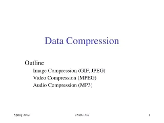
5. Data compression implies sending or storing a smaller number of bits. Although many methods are used for this purpose, in general these methods can be divided into two broad categories: lossless and lossy methods. Figure 15.1 Data compression methods

6. Data compression techniques are broadly classified into lossless and lossy. Lossless techniques enable exact reconstruction of the original document from the compressed information. Exploit redundancy in data Applied to general data Examples: Run-length, Huffman, LZ77, LZ78, and LZW Lossy compression - reduces a file by permanently eliminating certain redundant information Exploit redundancy and human perception Applied to audio, image, and video Examples: JPEG and MPEG Lossy techniques usually achieve higher compression rates than lossless ones but the latter are more accurate. Lossless and Lossy Compression Techniques

7. Lossless techniques are classified into static, adaptive (or dynamic), and hybrid. In a static method the mapping from the set of messages to the set of codewords is fixed before transmission begins, so that a given message is represented by the same codeword every time it appears in the message being encoded. Static coding requires two passes: one pass to compute probabilities (or frequencies) and determine the mapping, and a second pass to encode. Examples: Static Huffman Coding In an adaptive method the mapping from the set of messages to the set of codewords changes over time. All of the adaptive methods are one-pass methods; only one scan of the message is required. Examples: LZ77, LZ78, LZW, and Adaptive Huffman Coding An algorithm may also be a hybrid, neither completely static nor completely dynamic. Classification of Lossless Compression Techniques

8. Compression tool examples: winzip, pkzip, compress, gzip General compression formats: .zip, .gz Common image compression formats: JPEG, JPEG 2000, BMP, GIF, PCX, PNG, TGA, TIFF, WMP Common audio (sound) compression formats: MPEG-1 Layer III (known as MP3), RealAudio (RA, RAM, RP), AU, Vorbis, WMA, AIFF, WAVE, G.729a Common video (sound and image) compression formats: MPEG-1, MPEG-2, MPEG-4, DivX, Quicktime (MOV), RealVideo (RM), Windows Media Video (WMV), Video for Windows (AVI), Flash video (FLV) Compression Utilities and Formats

9. 15-1 LOSSLESS COMPRESSION In lossless data compression, the integrity of the data is preserved. The original data and the data after compression and decompression are exactly the same because, in these methods, the compression and decompression algorithms are exact inverses of each other: no part of the data is lost in the process. Redundant data is removed in compression and added during decompression. Lossless compression methods are normally used when we cannot afford to lose any data.

10. Run-length encoding Run-length encoding is probably the simplest method of compression. It can be used to compress data made of any combination of symbols. It does not need to know the frequency of occurrence of symbols and can be very efficient if data is represented as 0s and 1s. The general idea behind this method is to replace consecutive repeating occurrences of a symbol by one occurrence of the symbol followed by the number of occurrences. The method can be even more efficient if the data uses only two symbols (for example 0 and 1) in its bit pattern and one symbol is more frequent than the other.

11. Figure 15.2 Run-length encoding example

12. Figure 15.3 Run-length encoding for two symbols

13. The following string: BBBBHHDDXXXXKKKKWWZZZZ can be encoded more compactly by replacing each repeated string of characters by a single instance of the repeated character and a number that represents the number of times it is repeated: 4B2H2D4X4K2W4Z Here "4B" means four B's, and 2H means two H's, and so on. Compressing a string in this way is called run-length encoding. As another example, consider the storage of a rectangular image. As a single color bitmapped image, it can be stored as: The rectangular image can be compressed with run-length encoding by counting identical bits as follows: 0, 40 0, 40 0,10 1,20 0,10 0,10 1,1 0,18 1,1 0,10 0,10 1,1 0,18 1,1 0,10 0,10 1,1 0,18 1,1 0,10 0,10 1,20 0,10 0,40 Run-length encoding The first line says that the first line of the bitmap consists of 40 0's. The third line says that the third line of the bitmap consists of 10 0's followed by 20 1's followed by 10 more 0's, and so on for the other lines

14. Huffman coding Huffman coding assigns shorter codes to symbols that occur more frequently and longer codes to those that occur less frequently. For example, imagine we have a text file that uses only five characters (A, B, C, D, E). Before we can assign bit patterns to each character, we assign each character a weight based on its frequency of use. In this example, assume that the frequency of the characters is as shown in Table 15.1.

15. Figure 15.4 Huffman coding

16. A character’s code is found by starting at the root and following the branches that lead to that character. The code itself is the bit value of each branch on the path, taken in sequence. Figure 15.5 Final tree and code

17. Encoding Let us see how to encode text using the code for our five characters. Figure 15.6 shows the original and the encoded text. Figure 15.6 Huffman encoding

18. Decoding The recipient has a very easy job in decoding the data it receives. Figure 15.7 shows how decoding takes place. Figure 15.7 Huffman decoding

19. Lempel Ziv encoding Lempel Ziv (LZ) encoding is an example of a category of algorithms called dictionary-based encoding. The idea is to create a dictionary (a table) of strings used during the communication session. If both the sender and the receiver have a copy of the dictionary, then previously-encountered strings can be substituted by their index in the dictionary to reduce the amount of information transmitted.

20. Compression In this phase there are two concurrent events: building an indexed dictionary and compressing a string of symbols. The algorithm extracts the smallest substring that cannot be found in the dictionary from the remaining uncompressed string. It then stores a copy of this substring in the dictionary as a new entry and assigns it an index value. Compression occurs when the substring, except for the last character, is replaced with the index found in the dictionary. The process then inserts the index and the last character of the substring into the compressed string.

21. Figure 15.8 An example of Lempel Ziv encoding

22. Decompression Decompression is the inverse of the compression process. The process extracts the substrings from the compressed string and tries to replace the indexes with the corresponding entry in the dictionary, which is empty at first and built up gradually. The idea is that when an index is received, there is already an entry in the dictionary corresponding to that index.

23. Figure 15.9 An example of Lempel Ziv decoding

24. 15-2 LOSSY COMPRESSION METHODS Our eyes and ears cannot distinguish subtle changes. In such cases, we can use a lossy data compression method. These methods are cheaper—they take less time and space when it comes to sending millions of bits per second for images and video. Several methods have been developed using lossy compression techniques. JPEG (Joint Photographic Experts Group) encoding is used to compress pictures and graphics, MPEG (Moving Picture Experts Group) encoding is used to compress video, and MP3 (MPEG audio layer 3) for audio compression.

25. Image compression – JPEG encoding Image can be represented by a two-dimensional array (table) of picture elements (pixels). A grayscale picture of 307,200 pixels is represented by 2,457,600 bits, and a color picture is represented by 7,372,800 bits. In JPEG, a grayscale picture is divided into blocks of 8 × 8 pixel blocks to decrease the number of calculations because, as we will see shortly, the number of mathematical operations for each picture is the square of the number of units.

26. Figure 15.10 JPEG grayscale example, 640 × 480 pixels

27. The whole idea of JPEG is to change the picture into a linear (vector) set of numbers that reveals the redundancies. The redundancies (lack of changes) can then be removed using one of the lossless compression methods we studied previously. A simplified version of the process is shown in Figure 15.11. Figure 15.11 The JPEG compression process

28. Discrete cosine transform (DCT) In this step, each block of 64 pixels goes through a transformation called the discrete cosine transform (DCT). The transformation changes the 64 values so that the relative relationships between pixels are kept but the redundancies are revealed. P(x, y) defines one value in the block, while T(m, n) defines the value in the transformed block.

29. To understand the nature of this transformation, let us show the result of the transformations for three cases. Figure 15.12 Case 1: uniform grayscale

30. Figure 15.13 Case 2: two sections

31. Figure 15.14 Case 3: gradient grayscale

32. Quantization After the T table is created, the values are quantized to reduce the number of bits needed for encoding. Quantization divides the number of bits by a constant and then drops the fraction. This reduces the required number of bits even more. In most implementations, a quantizing table (8 by 8) defines how to quantize each value. The divisor depends on the position of the value in the T table. This is done to optimize the number of bits and the number of 0s for each particular application.

33. Compression After quantization the values are read from the table, and redundant 0s are removed. However, to cluster the 0s together, the process reads the table diagonally in a zigzag fashion rather than row by row or column by column. The reason is that if the picture does not have fine changes, the bottom right corner of the T table is all 0s. JPEG usually uses run-length encoding at the compression phase to compress the bit pattern resulting from the zigzag linearization.

34. Figure 15.15 Reading the table

35. Video compression – MPEG encoding The Moving Picture Experts Group (MPEG) method is used to compress video. In principle, a motion picture is a rapid sequence of a set of frames in which each frame is a picture. In other words, a frame is a spatial combination of pixels, and a video is a temporal combination of frames that are sent one after another. Compressing video, then, means spatially compressing each frame and temporally compressing a set of frames.

36. Spatial compression The spatial compression of each frame is done with JPEG, or a modification of it. Each frame is a picture that can be independently compressed. Temporal compression In temporal compression, redundant frames are removed. When we watch television, for example, we receive 30 frames per second. However, most of the consecutive frames are almost the same. For example, in a static scene in which someone is talking, most frames are the same except for the segment around the speaker’s lips, which changes from one frame to the next.

37. Figure 15.16 MPEG frames

38. Audio compression Audio compression can be used for speech or music. For speech we need to compress a 64 kHz digitized signal, while for music we need to compress a 1.411 MHz signal. Two categories of techniques are used for audio compression: predictive encoding and perceptual encoding.

39. Predictive encoding In predictive encoding, the differences between samples are encoded instead of encoding all the sampled values. This type of compression is normally used for speech. Several standards have been defined such as GSM (13 kbps), G.729 (8 kbps), and G.723.3 (6.4 or 5.3 kbps). Detailed discussions of these techniques are beyond the scope of this book. Perceptual encoding: MP3 The most common compression technique used to create CD-quality audio is based on the perceptual encoding technique. This type of audio needs at least 1.411 Mbps, which cannot be sent over the Internet without compression. MP3 (MPEG audio layer 3) uses this technique.

40. Relations for relationship sets For each relationship set in the E-R diagram, we create a relation (table). This relation has one column for the key of each entity set involved in this relationship and also one column for each attribute of the relationship itself if the relationship has attributes (not in our case).

41. Distinguish between lossless and lossy compression. • Describe run-length encoding and how it achieves compression. • Describe Huffman coding and how it achieves compression. • Describe Lempel Ziv encoding and the role of the dictionary in encoding and decoding. • Describe the main idea behind the JPEG standard for compressing still images. • Describe the main idea behind the MPEG standard for compressing video and its relation to JPEG. • Describe the main idea behind the MP3 standard for compressing audio.