Download
1 / 22
220 likes | 415 Vues
ECE4270 Fundamentals of DSP Lecture 8 Discrete-Time Random Signals I. School of Electrical and Computer Engineering Center for Signal and Image Processing Georgia Institute of Technology. Overview of Lecture 8. Announcement What is a random signal? Random process Probability distributions

E N D
ECE4270Fundamentals of DSPLecture 8Discrete-Time Random Signals I School of Electrical and Computer Engineering Center for Signal and Image Processing Georgia Institute of Technology
Overview of Lecture 8 • Announcement • What is a random signal? • Random process • Probability distributions • Averages • Mean, variance, correlation functions • The Bernoulli random process • MATLAB simulation of random processes
Announcement • Quiz # 1 • Monday Feb. 20 (at the class hour). • Open book and notes (closed HWKs). • Coverage: Chapters 2 and 3.
What is a random signal? • Many signals vary in complicated patterns that cannot easily be described by simple equations. • It is often convenient and useful to consider such signals as being created by some sort of random mechanism. • Many such signals are considered to be “noise”, although this is not always the case. • The mathematical representation of “random signals” involves the concept of a random process.
Random Process • A random process is an indexed set of random variables each of which is characterized by a probability distribution (or density) • and the collection of random variables is characterized by a set of joint probability distributions such as (for all n and m),
Sample function Sample function Ensemble of Sample Functions • We imagine that there are an infinite set of possible sequences where the value at n is governed by a probability law. We call this set an ensemble.
TotalArea = 1 Uniform Distribution
Averages of Random Processes • Mean (expected value) of a random process • Expected value of a function of a random process • In general such averages will depend upon n. However, for a stationary random process, all the first-order averages are the same; e.g.,
More Averages • Mean-squared (average power) • Variance
Joint Averages of Two R.V.s • Expected value of a function of two random processes. • Two random processes are uncorrelated if • Statistical independence implies • Independent random processes are also uncorrelated.
Correlation Functions • Autocorrelation function • Autocovariance function • Crosscorrelation function • Crosscovariance function
Stationary Random Processes • The probability distributions do not change with time. • Thus, mean and variance are constant • And the autocorrelation is a one-dimensional function of the time difference.
Time Averages • Time-averages of a random process are random variables themselves. • Time averages of a single sample function
Ergodic Random Processes • Time-averages are equal to probability averages • Estimates from a single sample function
Histogram • A histogram shows counts of samples that fall in certain “bins”. If the boundaries of the bins are close together and we use a sample function with many samples, the histogram provides a good estimate of the probability density function of an (assumed) stationary random process.
Sample function Bernoulli Random Process • Suppose that the signal takes on only two different values +1 or -1 with equal probability. • Furthermore, assume that the outcome at time n is independent of all other outcomes.
Bernoulli Process (cont.) • Mean: • Variance: • Autocorrelation: ( are assumed independent)
MATLAB Bernoulli Simulation • MATLAB’s rand( ) function is useful for such simulations. • >> d = rand(1,N); %uniform dist. Between 0 & 1 • >> k = find(x>.5); %find +1s • >> x = -ones(1,N); %make vector of all -1s • >> x(k) = ones(1,length(k)); %insert +1s • >> subplot(211); han=stem(0:Nplt-1,x(1:Nplt)); • >> set(han,’markersize’,3); • >> subplot(212); hist(x,Nbins); hold on • >> stem([-1,1],N*[.5,.5],'r*'); %add theoretical values