Discrete-Time Signals and Systems

ENGR 4333/5333: Digital Signal Processing Discrete-Time Signals and Systems Chapter 4 Dr. Mohamed Bingabr University of Central Oklahoma

Outline • Operations on the Independent DT Variable • DT Signal Models • DT Signal Classifications • DT Systems and Examples • DT System Properties • Digital Resampling

Connections between Continuous and Discrete = e-t = e-0.1n = e-nT x(t) = (0.368)n T= 0.1 t Single-input, single-output systems (SISO) Single-input, multiple-output systems (SIMO) Multiple-input, single-output systems (MISO) Multiple-input, multiple-output systems (MIMO)

Operation on the Independent DT Variable DT Time Shifting

Operation on the Independent DT Variable DT Time Reversal Replace nby -n Drill 4.3: Show that x[−n − m] can be obtained from x[n] by first right shifting x[n] by m units and then time reversing this shifted signal.

DT Time Scaling: Sampling Rate Conversion Compression, Downsampling, and Decimation Replacing n with Mnin x[n] compresses the signal by factor M to produce x↓[n] = x[Mn]. This means that x[Mn] selects every M th sample of x[n] and deletes all the samples in between. Expansion, Upsampling, and Interpolation An interpolated signal is generated in two steps: an expansion followed by filtering. Expand x[n] by an integer factor L to obtain the expanded signal x↑[n]

Drill 4.5: Sample Interpolation A signal x[n] = sin(2πn/4) is expanded by L = 2 to produce x↑[n]. Next, this signal is interpolated according to xi[n] = 0.5x↑[n − 1] + x↑[n] + 0.5x↑[n + 1]. Sketch x[n], x↑[n], and xi[n], and comment on the overall quality of the signal interpolation.

4.2Signal Models

DT Signal Models: Unit Step Function u[n] Example: Plot u[n] - u[n-10]

DT Unit Impulse Function [n] Multiplication by a DT Impulse [n] The Sampling Property Relationship between [n] and u[n]

Example Describe the signal x[n] shown below by a single expression, valid for all n, comprised of unit impulse and step functions

DT Exponential Function zn Sampling Where z = esT and esTn = zn est z will be real if s is real and complex if s is complex such as and z Letting r = |z| = and Ω =  z = so that z = rejΩ, the following functions are special cases of zn:

DT Exponential Function zn

DT Exponential Function znin the Complex Plane z The fundamental band (BW) Map to a unit circle. Any frequency outside it will be aliased as lower frequency in the fundamental band The s-plane imaginary axis becomes the z-plane unit circle |z| = 1.

Example Consider the DT exponential Re {zn}obtained from sampling the signal Re {est}with T = 1. Using z = esT, plot Re {zn}, as well as Re{est}for reference, over −5 ≤ n ≤ 5 for the cases s = −0.1 and s = −0.1+ j2π. Comment on the results. Note: Many points in the s-plane maps to one point in the z-plane (aliasing). B =1Hz so fs should be 2 and T= 0.5 sec. t = linspace(-5.5,5.5,1001); n = (-5:5); T = 1; s = -0.1+1j*0; z = exp(s*T); subplot(121); stem(n,real(z.^n)); line(t/T,real(exp(s*t))); s = -0.1+1j*2*pi; z = exp(s*T); subplot(122); stem(n,real(z.^n)); line(t/T,real(exp(s*t)));

DT Sinusoid A DT sinusoid frequency must meet the following constrains: cos(ωt)  cos(ωTn)  cos(2π f/Fsn)  cos(Ω n) f Fs/2 Ω  The unit of Ω is radians per sample The unit of F is cycle per sample Ω = ej|Ω|n e−j|Ω|n If r = 1 If we sample below the Nyquist rate then Ω > and the apparent frequency will be

Shifting in the CT produces a shifted identical signal. Shifting in the DT produces different samples if the shift is not a multiple integer of Ω. x[n] x[n - 2.5] Samples of x[n] will not be the same as samples of x[n - 2.5] shafted by 2.5 units

The Apparent Laziness of DT Exponential Our Eyes acts like a lowpass filter and we will not see the fast motion in the counterclockwise direction. We will see slower motion in the clockwise direction. The actual frequency is  + x but it will appear as  - x. Example: Express the following signals in terms of (positive) apparent frequency |Ωa|: (a) cos(0.5πn + θ) (b) cos(1.6πn + θ) (c) sin(1.6πn + θ) (d) cos(2.3πn + θ) (e) cos(34.6991n + θ)

4.3DT Signal Classification

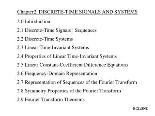
DT Signal Classifications 1. causal, noncausal, and anti-causal signals, 2. real and imaginary signals, 3. even and odd signals, 4. periodic and aperiodic signals, and 5. energy and power signals. Causal, noncausal, and anti-causal signals, Causal x[n] = 0 for n < 0 Noncausal is a signal that have values at positive and negative value of n Anti-causal x[n] = 0 for n 0

DT Signal Classifications Method to extract the Re and Img Real and Imaginary DT Signals Real x[n] = x[n]* Imaginary x[n] = - x[n]* Even and Odd DT Signals Even x[n] = x[-n] Odd x[n] = - x[-n]

DT Signal Classifications Conjugate Symmetries (Hermitian) Conjugate Symmetric x[n] = x*[-n] Conjugate Antisymmetric x[n] = - x*[-n] Periodic and Aperiodic DT Signals N-periodic x[n] = x[n - N] for all n. The smallest value of N that satisfy periodicity is called the fundamental period No. The fundamental frequency Fo = 1 / No or Ωo = 2 /No

DT Signal Classifications Cont. freq. cycles/sec Dig. freq. cycles/samples Periodicity of Sinusoidal Signal cos(2ft)  cos(2fnT)  cos (2 n)  cos (2 n)  cos (Ωn) samples/sec For the above to be periodic , where m is an integer. The fundamental period No of a DT sinusoid is easily determined by writing F in the reduced form, where the numerator and denominator are coprime.

Example a) Periodic, F = 3/15 = 1/5, so No = 5 b) Not periodic, F cannot be expressed as rational number. c) Periodic, F = 1/5.5 = 10/55 = 2/11, so No = 11

DT Signal Classifications DT Energy Signals DT Power Signal For No-periodic signal

Example

4.4DT Systems and Examples

DT Systems and Examples Discrete-time systems process discrete-time signals (inputs) to yield another set of discrete time signals (outputs). Operator H is used to represent the system function. The four major blocks in any DT systems are Adder Scalar Multiplier Delay Branch Node

Example Determine the non-recursive and recursive input-output equations of a cash register, where the input x[n] is the price of the nth item and the output y[n] is the total value of all n items entered in the register. Provide a block diagram representation of the system. Non-recursive System: Output is calculated from current and previous inputs. Recursive System: Output is calculated from previous output and current input.

DT Systems and Examples Delay and Advance Forms Delay Advance Advance form is noncausal and unrealizable, but can be used to predict future value if we are welling to wait for the output. The Accumulator Accumulator is analogous to the integrator in continuous-time system

Example A person makes a deposit (the input) in a bank regularly at an interval of T = 1 month. The bank pays a certain interest on the account balance during the period T and mails out a periodic statement of the account balance (the output) to the depositor. Find the equation relating the output y[n] (the balance) to the input x[n] (the deposit). Assuming that a person invests $100 monthly starting at n = 1 and earns a 0.5% monthly interest rate, how much money is earned at n = 100? Provide a block diagram representation of the system. Solution Let a1 = -(1 + r)

Example (Digital Differentiator) Design a discrete-time system to diﬀerentiate continuous-time signals. Construct a block diagram representation of the system, and investigate its response to a ramp input x(t) = tu(t). Suggest an appropriate sampling interval if this is used in an audio system where the input signal bandwidth is below 20 kHz. Solution First order difference system Backward difference Forward difference

Example (Digital Integrator) Design discrete-time systems to integrate continuous-time signals using (a) a backward-staircase approximation, (b) a forward-staircase approximation, and (c) a trapezoidal approximation. Construct a block diagram representation for each system. Solution Backward Forward Trapezoidal

Example (Digital Integrator) Backward Forward Trapezoidal

Order and General Form of Difference Equations Just as the highest-order derivative of the input or output represents the order of a differential equation, the highest-order difference of the input or output represents the order of a difference equation. Order is reflective of system complexity. For CT systems, order indicates the number of energy storage elements, such as capacitors and inductors, required for implementation. For DT systems, order indicates the required amount of memory.

Order and General Form of Difference Equations Example Assuming a sampling interval T = 0.1, determine a difference equation model for the differential equation with initial conditions y(0) = 0 and = 10. Answer:

Advantage of Digital Signal Processing • Digital systems can tolerate considerable variation in signal values and, hence, are less sensitive to changes in the component parameter values. • Digital systems are extremely flexible and easy to implement. • Even in the presence of noise, reproduction with digital messages is extremely reliable, often without any deterioration whatsoever. • Digital signals are easily and inexpensively stored electronically, without any loss of signal quality. • Digital filters can be easily time shared and therefore can serve a number of inputs simultaneously. • Digital implementation permits the use of a wide variety of hardware options, including computers and microprocessors, DSPs. • Disadvantage: Power consumption, limited frequency range and resolution, system complexity.

4.5DT System Properties

DT System Properties Time Invariance Example: A system is described by the equation y[n] = e-n x[n}. Is the system time invariant system?

DT System Properties Linearity If then

The Zero-State Response of an LTID Systems Example: Consider an LTID system that has an impulse response h[n] = 2−nu[n]. Using the input x[n] = u[n] − u[n − 10], determine and sketch the zero-state response of this system over −10 ≤ n ≤ 20. h = @(n) 2.^(-n).*(n>=0); y = @(n) 0; for m = 0:9, y = @(n) y(n)+h(n-m); end n = -10:20; stem(n,y(n)); xlabel('n'); ylabel('y[n]');

DT System Properties Causality: A causal system is one for which the output at any instant n = n0 depends only on the value of the input x[n] for n ≤ n0. h[n] = 0 for n < 0 Example: The general-order difference equation in advance form is . Show that for the system to be causal K L. If L = K and replace n + K by n then the general causal difference equation is

Direct Form 1 Realization of a Kth order Difference Equation

DT System Properties Stability External Stability (BIBO) |y[n]|  Ky <  if |x|  Kx <  Internal Stability (asymptotic and marginal stability): depends on the parameter of the system (Chapter 5) Memory If the output of a discrete-time system depends on input values other than the present one, then the system has memory. Systems with memory are also called dynamic systems. A system without memory is called a memoryless, instantaneous, or static system. Invertibility A discrete-time system H is invertible if an inverse system Hi exists such that the cascade of H and Hi results in an identity system (output equals input).

4.6Digital Resampling

Digital Resampling Combined with appropriate filtering, expansion and compression are the backbone operations for multirate systems. These operations provide an effective means to digitally alter the sampling rate of a DT signal, even by non-integer factors. Compressor (Downsampling ) Antialiasing Filter Expander (Upsampling) Interpolator Filter Cascade ordering of compression and expansion systems does matter in certain cases, see next example.

Example: Consider the signal x[n] = cos(πn), whose frequency is the highest possible without aliasing. Determine the output when this signal is applied to the following systems: (a) An upsample by L = 4 operation followed by a downsample by M = 2 operation. (b) A downsample by M = 2 operation followed by an upsample by L = 4 operation. (c) An upsample by L = 3 operation followed by a downsample by M = 2 operation. (d) A downsample by M = 2 operation followed by an upsample by L = 3 operation. DownsampleM = 2Upsample L = 4 UpsampleL = 4  DownsampleM = 2

DownsampleM = 2Upsample L = 3 UpsampleL = 3  DownsampleM = 2 if L and M are coprime, which is to say they have no common factors other than 1, then the operations of expansion and compression commute. In practice ordering may change aliasing, and speed of operation.

Discrete-Time Signals and Systems