Download
1 / 72
740 likes | 1.32k Vues
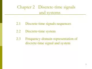
Chapter 2 Discrete-time signals and systems. 2.1 Discrete-time signals:sequences. 2.2 Discrete-time system. 2.3 Frequency-domain representation of discrete-time signal and system. 2.1 Discrete-time signals:sequences. 2.1.1 Definition.

E N D
Chapter 2 Discrete-time signals and systems 2.1 Discrete-time signals:sequences 2.2 Discrete-time system 2.3 Frequency-domain representation of discrete-time signal and system
2.1 Discrete-time signals:sequences 2.1.1 Definition 2.1.2 Classification of sequence 2.1.3 Basic sequences 2.1.4 Period of sequence 2.1.5 Symmetry of sequence 2.1.6 Energy of sequence 2.1.7 The basic operations of sequences
Enumerative representation Function representation 2.1.1 Definition EXAMPLE
0.5 2 1 0 0 -1 -0.5 -2 -1 -3 0 5 10 -2 0 2 4 6 Graphical representation
Generate and plot the sequence in MATLAB n=-1:5 x=[1,2,1.2,0,-1,-2,-2.5] stem(n,x, '.') n=0:9 y=0.9.^n.*cos(0.2*pi*n+pi/2) stem(n,y,'.')
EXAMPLE Sampling the analog waveform Figure 2.2
local Blowup Display the wav speech signal in COOLEDIT The whole waveform Display the wav speech signal in
2.1.2 Classification of sequence Right-side Left-side Two-side Finite-length Causal Noncausal
2.1.3 Basic sequences 1. Unit sample sequence 2.The unit step sequence 3.The rectangular sequence
For convenience, sinusoidal signals are usually expressed by exponential sequences. The relationship between ω and Ω:
2.1.5 Symmetry of sequence Conjugate-symmetric sequence Conjugate-antisymmetric sequence
EXAMPLE n=[-5:5]; x=[0,0,0,0,0,1,2,3,4,5,6]; xe=(x+fliplr(x))/2 ; xo=(x-fliplr(x))/2; subplot(3,1,1) stem(n,x) subplot(3,1,2) stem(n,xe) subplot(3,1,3) stem(n,xo) Real sequences can be decomposed into two symmetrical sequences.
EXAMPLE Complex sequences can be decomposed into two symmetrical sequences. n=[-5:5]; x=zeros(1,11); x((n>=0)&(n<=5))=(1+j).^[0:5] xe=(x+conj(fliplr(x)))/2; xo=(x-conj(fliplr(x)))/2 subplot(3,2,1); stem(n,real(x)) subplot(3,2,2); stem(n,imag(x)) subplot(3,2,3); stem(n,real(xe)) subplot(3,2,4); stem(n,imag(xe)) subplot(3,2,5); stem(n,real(xo)) subplot(3,2,6); stem(n,imag(xo))
Original speech sequences Original music sequence sequences after scalar multiplication sequences after vector addition sequences after vector multiplication echo
n=[-4:2] ; x=[1,-2,4,6,-5,8,10] ; %x1[n]=x[n+2] n1=n-2; x1=x; %x2[n]=x[n-4] n2=n+4; x2=x; %y[n] m=[min(min(n1),min(n2)): max(max(n1),max(n2))] ; y1=zeros(1,length(m)) ; y2=y1; y1((m>=min(n1))&(m<=max(n1)))=x1;y2((m>=min(n2))&(m<=max(n2)))=x2; y=3*y1+y2; stem(m,y) Output:y =3 -6 12 18 -15 24 31 -2 4 6 -5 8 10
7.convolution sum: steps:turnover, shift, vector multiplication, addition
EXAMPLE nx=0:10; x=0.5.^nx; nh=-1:4; h=ones(1,length(nh)) y=conv(x,h); stem([min(nx)+min(nh):max(nx)+max(nh)],y)
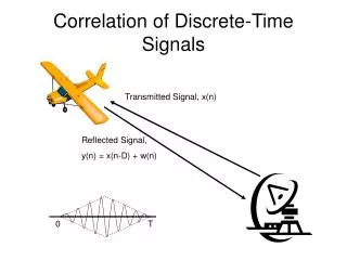
8.crosscorrelation: aotocorrelation:
2.1 summary • 2.1.1 Definition • 2.1.2 Classification of sequence • 2.1.3 Basic sequences • 2.1.4 Period of sequence • 2.1.5 Symmetry of sequence • 2.1.6 Energy of sequence • 2.1.7 The basic operations of sequences
requirements:judge the period of sequence ; • calculate convolution with graphical • and analytical evaluation . • key: convolution
2.2 Discrete-time system 2.2.1 Definition:input-output description of systems 2.2.2 Classification of discrete-time system 2.2.3 Linear time-invariant system(LTI) 2.2.4 Linear constant-coefficient difference equation 2.2.5. Direct implementation of discrete-time system
2.2.1 definition:input-output description of systems the impulse response
2.2.2 classification of discrete-time system 1.Memoryless (static) system the output depends only on the current input. 2.Linear system 3.Time-invariant system: 4.Causal system: the output does not depend on the latter input. 5.Stable system:
2.2.3 linear time-invariant system(LTI) How to get h[n] from the input and output:
the impulse response in LTI EXAMPLE
h[n] Properties of LTI Figure 2.12
classification of linear time-invariant system IIR: h[n]’s length is infinite the latter input the former input FIR must be stable。
2.2.4 linear constant-coefficient difference equation 1.relation with input-output description and convolution For IIR,the latter two are consistent. EXAMPLE input-output description convolution description infinite items,unrealizable difference equation description Finite items, realizable
EXAMPLE For FIR,the followings are consistent input-output description and difference equation description (non-recursion) Convolution description Another difference equation description,recursion,lower rank For FIR and IIR,difference equations are not exclusive.
2.Recursive computation of difference equations: For IIR, there needs N initial conditions , then ,the solution is unique. For FIR, there needs no initial conditions. With initial-rest conditions (linear, time invariant, and causal), the solution is unique. EXAMPLE
3.computation of difference equations with homogeneous and particular solution
2.2.5. Direct implementation of discrete-time system EXAMPLE
EXAMPLE The matlab codes on the direct realization of LTI B=1; A=[1,-1] n=[0:100]; x=[n>=0]; y=filter(B,A,x); stem(n,y); axis([0,20,0,20])