Download
1 / 126
1.28k likes | 1.34k Vues
Learn how to mathematically represent discrete-time signals and systems in the time and frequency domains. Topics include classification of signals, time-domain representation, and MATLAB implementation.

E N D
To understand the theory of digital signal processing and design of discrete-time systems, we need to know how to mathematically represent discrete-time signals and systems. Such representations can be either in the time-domain or in the frequency domain.
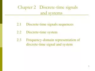
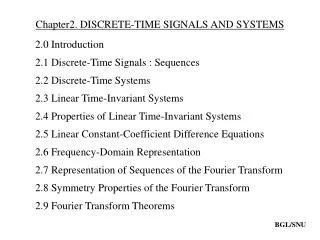
Content • Introduction • Discrete-time signals • Discrete-time systems • Time-domain characterization of LTI discrete-time systems • Digitalization of Analog Digital
1.1 Introduction • A signal is a function of independent variables. Depending on the nature of the independent variables and value of the function defining the signal, various types of signals can be defined.
1.1 Introduction • Classification of signals 1. Analog signal—A continuous-time signal with a continuous amplitude. 2. Digital signal—A discrete-time signal with discrete-valued amplitudes represented by a finite number of digits.
1.1 Introduction • Classification of signals 3. Sampled-data signal--A discrete-time signal with a continuous-valued amplitude. 4. Quantized boxcar signal—A continuous-time signal with discrete-valued amplitudes represented by a finite number of digits.
1.1 Introduction • Note: A continuous-time signal is defined at every instant of time. On the other hand, a discrete-time signal takes certain numerical values at specified discrete instants of time, and between these specified instants of time, the signal is not defined.
1.1 Introduction • Classification of signals • Depending on the number of independent variable, the signal can be classified as • one-dimensional signal (speech) • two-dimensional signal (image) • multidimensional signal (video)
1.1 Introduce • Classification of Signals • Another classification of signals that depends on the certainty by which the signal can be uniquely described. • Deterministic signal • Random signal
1.2 Discrete-time signals • Time-Domain representation In digital processing, a discrete-time signal can be represented as a sequence of numbers called samples, with the independent time variable represented as an integer in range from -∞ to +∞.
1.2 Discrete-time signals • Time-Domain representation If a discrete-time signal is written as a sequence of numbers inside braces, the location of the sample value associated with the time index n=0 is indicated by an arrow under it. The sample values to its right are for positive values of n, and the sample values to its left are for negative values of n.
1.2 Discrete-time signals • Time-Domain representation The graphical representation of a sequence {x[n]} with real-valued samples is illustrated in Figure 2.1.
1.2 Discrete-time signals • Time-Domain representation In some applications, a discrete-valued sequence {x[n]} is generated by periodically sampling a continuous-time signal at uniform time intervals T is called the sampling interval or sampling period, the reciprocal of T, denoted as , is called the sampling frequency
1.2 Discrete-time signals • Time-Domain representation
1.2 Discrete-time signals • Time-Domain representation • Note: • It should be noted that x[n] is defined only for integer values of n and undefined for noninteger values of n. • It should be noted that, whether or not a sequence {x[n]} has been obtained by sampling, the quantity x[n] is called the nth sample of the sequence.
1.2 Discrete-time signals • Time-Domain representation 3 .For a sequence {x[n]}, the nth sample value can, in general, take any real or complex value. If x[n] is real for all values of n, then {x[n]} is a real sequence. On the other hand, if nth sample value is complex for one or more values of n, then it is a complex sequence.
1.2 Discrete-time signals • Time-Domain representation By separating the real and imaginary parts of x[n], we can write a complex sequence {x[n]} as
1.2 Discrete-time signals • Time-Domain representation There are basically two types of discrete-time signals: sampled-data signals, in which the samples are continuous-valued, and digital signals, in which the samples are discrete-valued.
1.2 Discrete-time signals • MATLAB Implementation n=-5:5; x=sin(pi*n/5); stem(n,x,’.’); line([-5,6],[0,0]); axis([-5,6,-1.2,1.2]); xlabel(‘n’); ylabel((‘x(n)’)
1.2 Discrete-time signals • Typical sequences • We now consider several basic sequences that play important roles in the analysis and design of discrete-time systems. An arbitrary sequence can be expressed in terms of some of these basic sequences. • The most common basic sequences are the unit sample sequence, the unit step sequence, rectangle sequence,etc.
1.2 Discrete-time signals • Unit sample sequence The simplest and one of the most useful sequences is the unit sample sequence, often called the discrete-time impulse or the unit impulse. It is denoted by δ[n] and defined by
1.2 Discrete-time signals • Unit sample sequence
1.2 Discrete-time signals • Unit step sequence
1.2 Discrete-time signals • The unit sample and the unit step sequence are related as follows
1.2 Discrete-time signals • Rectangle sequence
1.2 Discrete-time signals • Rectangle sequence An application of the above sequence is in extracting all samples in the range N1<=n<=N2 of an infinite-length or very long length sequence x[n] and setting all other samples outside the above range to zero values by multiplying x[n] with RN(n).
1.2 Discrete-time signals • Real exponential sequence where a is a real.
1.2 Discrete-time signals • Sinusoidal sequence where
1.2 Discrete-time signals • periodic sequence A commonly encountered sequence is the real sinusoidal sequence with constant amplitude of the form
1.2 Discrete-time signals • periodic sequence For the periodic sequence with period N, if is an integer multiple of , that is or Then it is a periodic sequence of period
1.2 Discrete-time signals • periodic sequence If is a noninteger rational number, then the period will be a multiple of . If is not a rational number, then the sequence is aperiodic even through it has a sinusoidal envelop.
1.2 Discrete-time signals • Sequence generation using MATLAB • MATLAB includes a number of functions that can be used for signal generation. Some of these function of interest are exp, sin, cos, square, etc. • Some sequences can be generated by programming a MATLAB code fragments as follows:
1.2 Discrete-time signals • Sequence generation using MATLAB % Program P1_1 % Generation of a Unit Sample Sequence clf; n = -10:20; u = [zeros(1,10) 1 zeros(1,20)]; stem(n,u); xlabel('Time index n');ylabel('Amplitude'); title('Unit Sample Sequence'); axis([-10 20 0 1.2]);
1.2 Discrete-time signals % Program P1_2 % Generation of a complex exponential sequence clf; c = -(1/12)+(pi/6)*i; K = 2; n = 0:40; x = K*exp(c*n); subplot(2,1,1); stem(n,real(x)); xlabel('Time index n');ylabel('Amplitude'); title('Real part'); subplot(2,1,2); stem(n,imag(x)); xlabel('Time index n');ylabel('Amplitude'); title('Imaginary part');
1.2 Discrete-time signals % Program P1_3 % Generation of a real exponential sequence clf; n = 0:35; a = 1.2; K = 0.2; x = K*a.^n; stem(n,x); xlabel('Time index n');ylabel('Amplitude');
1.2 Discrete-time signals % Program P1_4 % Generation of a sinusoidal sequence n = 0:40; f = 0.1; phase = 0; A = 1.5; arg = 2*pi*f*n - phase; x = A*cos(arg); clf; % Clear old graph stem(n,x); % Plot the generated sequence axis([0 40 -2 2]); grid; title('Sinusoidal Sequence'); xlabel('Time index n'); ylabel('Amplitude'); axis;
1.2 Discrete-time signals • Representation of an arbitrary sequence • An arbitrary sequence can be represented in the time-domain as a weighted sum of a basic sequence and its delay versions. A commonly used sequence in the representation of an arbitrary sequence is unit sample sequence
1.2 Discrete-time signals For example, the sequence x[n] of the followed figure can be expressed as • Representation of an arbitrary sequence
1.2 Discrete-time signals • Operations on sequences • Various types of signal processing operations are employed in practice. In the case of discrete-time domain, the three most basic time-domain signal operations are scaling, delay, and addition. • In most cases, the operation defining a particular discrete-system is composed of some elementary operations that we describe next.
1.2 Discrete-time signals • Elementary operations • Scalar multiplication Addition • Time-shifting (delaying, advancing) Time-reversal, also called the folding operation
1.2 Discrete-time signals • Elementary operations • Product In some applications, the product operation is also known as modulation. • An application of the product operation is in forming a finite-length sequence from an infinite-length sequence by multiplying the latter with a finite-length sequence called a windows sequence.
1.2 Discrete-time signals • Combination of elementary operations In most applications, combinations of the above elementary operations are used.
EXAMPE Basic operations on sequences of equal lengths 1.2 Discrete-time signals Consider the following two sequences of length 5 defined for 0<=n<=4:
EXAMPE Basic operations on sequences of equal lengths 1.2 Discrete-time signals Several new sequences of length 5 generated from the above sequences are given by
As indicated by the above Example, operations on two or more sequences to generate a new sequence can be carried out if all sequences are of the same length and defined for the same range of the time indexn. However, if the sequences are not of equal length, all sequences can be made to have the same range of the time index n by appending zero-valued samples to the sequence of smaller lengths 1.2 Discrete-time signals
EXAMPE Basic operations on sequences of unequal lengths 1.2 Discrete-time signals Consider a sequence {g[n]} of length 3 defined for 0<=n<=2 given by