Chapter 2 Signals and Systems

1. Chapter 2 Signals and Systems Marcus Borengasser 8/24/10

2. Chapter 2 Introduction The object being imaged is an input signal – Typically a 3D signal • The imaging system is a transformation of the input signal to an output signal • The image produced is an output signal – Typically a 2D signal (an image, e.g. an X-ray) or a series of 2D signals (e.g. images from a CT scan)

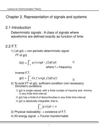
3. Chapter 2 Introduction Input signal: μ(x; y) is the linear attenuation coefficient for x-rays of a body component along a line • Imaging Process: integration over x variable: • Output signal: g(y)

4. Signals – Point Impulse The concept of a point source in one dimension is known as the 1-D point impulse, which is defined by the following two properties: The 2-D point impulse is analogously characterized by

5. Signals – Point Impulse

6. Signals – Line Impulse When calibrating medical imaging equipments, it is sometimes easier to use a line-like rather than a point-like object. For example, it may be easier to position a wire than a small bead to assess the resolution of a projection radiography system. For this reason, we would like a mathematical model for a line source. The set of points defined by Is a line whose unit normal is oriented at an angle θ relative to the x-axis and is at distance l from the origin. The line impulse associated with line L is given by

7. Signals – Comb and Sampling Functions As a first step toward characterizing sampling mathematically, the comb function is introduced. It is called the comb function because the set of shifted point impulses comprising it resembles the teeth of a comb. The 2-D comb is given by It is useful in signal sampling to space the point impulses in the comb function by amounts Δx in the x-direction, and Δy in the y-direction. This yields the samplings function, defined by

8. Signals – Rect and Sinc Functions Two signals that are frequently used in the study of medical imaging systems are the rect and sinc functions. The rect function is given by The sinc function is given by

9. Signals – Rect and Sinc Functions

10. Signals – Sinusoidal Signals Six instances of the sinusoidal signal s(x,y) = sin[2π(u0x + v0y], 0 ≤ x, y ≤ 1 for various values of the fundamental frequencies u0, v0. Notice that small values result in slow oscillations in the corresponding direction, whereas large values result in fast oscillations.

11. Signals – Separable Signals Separable signals form another class of continuous signals. A signal f(x,y) Is a separable signal if there exist two 1-D signals f1(x) and f2(y) such that A 2-D separable signal that is a function of two independent variables x and y can be separated into a product of two 1-D signals, one of which is only a function of x and the other only of y. Separable signals are limited, in the sense that they can only model signal variations independently in the x- and y-directions. Of major importance is the fact that operating on separable signals is much simpler than operating on purely 2-D signals, since for separable signals, 2-D operations reduce to simpler consecutive 1-D operations.

12. Systems – Linear Systems A simplifying assumption is that of linearity. A system S is a linear system if, when the input consists of a weighted summation of several signals, the output will also be a weighted summation of the responses of the system to each individual input signal.

13. Systems – Impulse Response

14. Systems – Shift Invariance An additional simplifying assumption is shift invariance. A system S is shift- invariant if an arbitrary translation of the input results in an identical translation in the output if

15. Systems – Connections of LSI Systems LSI systems can be stand-alone or connected with other LSI systems. Two types of connections are usually considered: (1) cascade or serialconnections; and (2) parallel connections.

16. Systems – Separable Systems Separable systems form an important class of LSI systems. As with separable signals, a 2-D LSI system with a point spread function (PSF, or impulse response function) h(x,y) is a separable system if there exist two 1-D systems with PSFs h1(x) and h2(y), such that h(x,y) = h1(x)h2(y), Calculation of the output of a 2-D separable system by using two 1-D steps in cascade.

17. Systems – Stable Systems A medical imaging system is stable if small inputs lead to outputs that do not diverge. Although there are many ways to characterize system stability, only consider BIBO stability. A system is a bounded-input bounded-output (BIBO) stable system if, when the input is a bounded signal – i.e. when for some finite B - there exists a finite B’ such that In which case the output will also be a bounded signal. It can be shown that an LSI system is a BIBO stable system if and only if its PSF is absolutely integrable, in which case

18. The Fourier Transform (FT) Besides decomposing a signal into point impulses, an alternative way to decompose a signal is in terms of complex exponential signals. It can be shown that, if then The signal F(u,v) is known as the (2-D) Fourier transform of f(x,y), whereas the signal decomposition below is known as the (2-D) inverse Fourier transform.

19. The Fourier Transform (FT) A Fourier transform is a linear transformation that allows calculation of the coefficients necessary for the sine and cosine terms to adequately represent the image. Because of the computational load in calculating the values for all the sine and cosine terms along with the coefficient multiplications, a highly efficient version of the discrete Fourier transform was developed - the Fast Fourier Transform.

20. The Fourier Transform (FT) Fourier transformations are typically used for the removal of noise such as striping, spots, or vibration in imagery by identifying periodicities (areas of high spatial frequency). Fourier editing can be used to remove regular errors in data such as those caused by sensor anomalies (e.g., striping). This analysis technique can also be used across bands as another form of pattern/feature recognition.

21. The Fourier Transform (FT) • The raster image generated by the Fourier transform calculation is not an • optimum image for viewing or editing. • Each pixel of a Fourier image is a complex number (i.e., it has two components • real and imaginary). For display as a single image, these components are • combined in a root-sum of squares operation. • Since the dynamic range of Fourier spectra vastly exceeds the range of a • typical display device, the Fourier magnitude calculation involves a logarithmic • function. • A Fourier image is symmetric about the origin (u,v = 0,0). If the origin is • plotted at the upper left corner, the symmetry is more difficult to see than if • the origin is at the center of the image. Therefore, in the Fourier magnitude image, • the origin is shifted to the center of the raster array.

22. The Fourier Transform (FT) Three images of decreasing spatial variation (from left to right) and the associated magnitude spectra.

23. The Fourier Transform (FT) - Filtering Homomorphic filtering is based upon the principle that an image may be modeled as the product of illumination and reflectance components: [NO REFLECTANCE ON MEDICAL IMAGES] I(x,y) = i(x,y) x r(x,y) where I(x,y) = image intensity at pixel x,y i(x,y) = illumination of pixel x,y (dominant at low frequencies) r(x,y) = reflectance at pixel x,y (dominant at higher frequencies) The illumination image is a function of lighting conditions. The reflectance image is a function of the object being imaged. A log function can be used to separate the two components (i and r) of the image: ln I(x,y) = ln i(x,y) + ln r(x,y)

24. The Fourier Transform (FT) - Filtering

25. Properties of the FT - Linearity The Fourier transform satisfies a number of useful properties. Most of them are used in both theory and applications to simplify calculations. If the Fourier transforms of two signals f(x,y) and g(x,y) are F(u,v) and G(u,v), respectively, then where a1 and a2 are two constants. This property can be extended to a linear combination of an arbitrary number of signals.

26. Properties of the FT - Translation If F(u,v) is the Fourier transform of a signal f(x,y), and if then In this case, and Therefore, translating a signal f(x,y) does not affect its magnitude spectrum but subtracts a constant phase of 2π (ux0+ vy0) at each frequency (u,v).

27. Sampling – Sampling Signal Model Continuous signals must be transformed into collections of numbers. This process, called discretization or sampling, means that only the representative signal values are retained. One way to do this is with a rectangular sampling scheme. According to this scheme, a 2-D continuous signal is replaced by a discrete signal whose values are the values of the continuous signal at the vertices of a 2-D rectangular grid. Δx and Δy are the sampling periods in the x and y directions, respectively. A coarse and a fine rectangular sampling scheme. Although coarse sampling results in fewer samples, it may not allow reconstruction of the original continuous signal.

28. End-of-Chapter Problems Problem 2.1 (a) Determine whether the following signal is separable. Problem 2.2 (b) Determine whether the following signal is periodic and, if it is, what Is the smallest period. So the smallest period is 1 in both x and y directions.

29. End-of-Chapter Problems Problem 2.5 show that an LSI system is BIBO stable if and only if its PSF is absolutely integrable.

30. End-of-Chapter Problems Problem 2.5 Continued

31. References Prince, J.L. and Links, J.M., 2006. Medical Imaging: Signals and Systems, Prentice Hall, 480 p.