Download
1 / 44
520 likes | 1.04k Vues
g(t) =. Chapter 2. Representation of signals and systems. 2.1 Introduction Deterministic signals : A class of signals where waveforms are defined exactly as function of time . 2.2 F.T. 1) Let g(t) = non-periodic deterministic signal F T of g(t) inverse F.T.

E N D
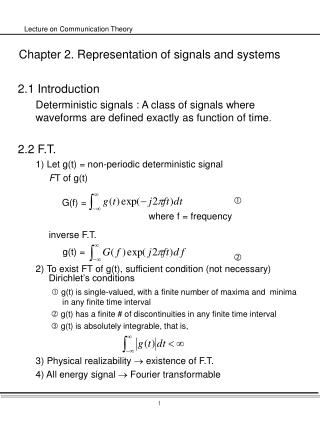
g(t) = Chapter 2. Representation of signals and systems • 2.1 Introduction • Deterministic signals : A class of signals where waveforms are defined exactly as function of time. • 2.2 F.T. • 1) Let g(t) = non-periodic deterministic signal • FT of g(t) • • inverse F.T. • • 2) To exist FT of g(t), sufficient condition (not necessary) Dirichlet’s conditions • g(t) is single-valued, with a finite number of maxima and minima in any finite time interval • g(t) has a finite # of discontinuities in any finite time interval • g(t) is absolutely integrable, that is, • 3) Physical realizability existence of F.T. • 4) All energy signal Fourier transformable G(f) = where f = frequency
2.2 Fourier Transform • 1. Notation • t : time [sec] • f : frequency [Hertz] • w= 2pf : angular frequency [radians/sec] • 식 G(f) = F [g(t)] • 식 g(t) = F-1[G(f)] • F, F-1 : linear operator • 2. Continuous Spectrum • 1) Continuous Spectrum G(f) = |G(f)| exp[j(f)] • |G(f)| : Continuous amplitude spectrum of g(t) • (f) : Continuous phase spectrum of g(t) • 2) For real-valued g(t) • G(f) = G*(f) = |G(-f)| = | G(f)| • (-f) = - (f) • Complex conjugation = conjugate symmetric • Real : y 축 대칭, symmetric • Imaginary : 원점 대칭, anti-symmetric g(t) G(f)
A AT -1/T 1/T 0 T/2 -T/2 • Ex1) Rectangular pulse • Def) rect(t) = 1 -1/2 < t < 1/2 • 0 |t| > 1/2 • g(t) = A rect (t/T) • • Def) sinc function • • G(f) = AT sinc (fT) • A rect(t/T) AT sinc (fT) • 3) Real Symmetric Real Symmetric • Ex2) exp(-at) u(t) • exp(at) u(-t) FT
2.3 Properties of the Fourier Transform • 1. Linearity (Superposition) • Let g1(t) G1(f) and g2(t) G2(f). • Then for all constants C1 and C2, we have • C1 g1(t) + C2 g2(t) C1 G1(f)+ C2 G2(f) • 2. Time Scaling • Let g(t) G(f). Then g(at) 1/|a| G(f/a) • when a=-1, g(-t) G(-f) • 3. Duality • If g(t) G(f), then G(t) g(-f) • 4. Time shifting • If g(t) G(f), then • g(t-t0) G(f)exp(-j2pft0) • 5. Frequency shifting • If g(t) G(f), then exp(j2pfct)g(t) G(f-fc) • where fc is a real constant • modulation theorem
|G(f)| g(t) -fc fc T • Ex5) RF pulse • g(t) =a rect(t/T)cos(2pfct) • G(f) = AT/2 {sinc[T(f-fc)] + sinc[T(f+fc)]} • 6. Area under g(t) • Ifg(t) G(f), then • 7. Area under G(f) • If g(t) G(f), then • 8. Differentiation in the Time Domain • Let g(t) G(f), and assume that the 1st derivative of g(t) is Fourier transformable. Then • n-th generalization Ex6) Gaussian pulse g(t) = exp(-pt2) exp(-pf2)
9. Integration in the Time Domain • Let g(t) G(f), then provided that G(0)=0, we have • 10. Conjugate Functions • If g(t) G(f), then for a complex-valued time function g(t), • we have g*(t) G*(-f), • when the asterisk denotes the complex conjugate operation <Corollary> g*(-t) G*(f) • 11. Multiplication in the Time Domain • (Multiplication Theorem) • Let g1(t) G1(f) and g2(t) G2(f), Then g1(t)g2(t) 12. Convolution in the Time Domain (Convolution Theorem) Let g1(t) G1(f) and g2(t) G2(f), Then g1(t) g2(t) G1(f)G2(f)
2.4 Rayleigh’s Energy Theorem • 1. Rayleigh’s Energy Theorem • E = linear transform • Ex9) E =
-1/T 1/T 0 Base-band Pass-band modulation 0 fc + 1/T fc BW = 2/T BW = 1/T 2 배 차이 2.5 The inverse relationship btw time and frequency • 1. Time과 frequency 관계 • 1) linear transform of FT • 2) Time Frequency wide low narrow high cannot specify arbitrary function of time and frequency. • 3)Strictly limited in time infinite in freq. infinite in time strictly band-limited in freq. cannot be strictly limited in both time and freq. • 2. Bandwidth • 1) def) extent of significant spectral content of the signal for signal positive frequencies • 2) strictly band-limited 경우가 아닐 경우의 definitions • BW = Main lobe bounded by well-defined nulls
Wrms 3 dB Bandwidth : of its peak value rms(root mean square) BW (장점) mathematical evaluation (단점) not easily measurable in lab • 3. Time-Bandwidth Product • 1) for base-band sync function • = (duration T) • (BW of main lobe = 1/T) =1 • 2) Trms Wrms 1/4 • “ = “ when Gaussian pulse • 2.6 Dirac Delta Function • 1. Definition • (t) = 0, t 0 • (t) is even function of t • 2. Shifting property
f g(t) G(f) f 1.0 t f • 3. Replication property g(t) (t) = g(t) • 4. Fourier Transform F [(t)] = 1 • 5. Applications of the Delta Function • 1) dc signal 1 (f) • 2) Complex Exponential Function • exp(j2fct) (f-fc) • 3) Sinusoidal Functions • cos (2fct) = 1/2 [exp (j2fct) + exp (-j2fct)] • 1/2 [(f-fc) + (f+fc)] • Sin(2fct) 1/2j [(f-fc) - (f+fc)]
g(t) t g(t) + 1.0 t 0 - 1.0 |G(f)| |G(f)| 1/2 f f 0 • 4) signum Function • sgn[t] = +1, t > 0 • 0, t = 0 • -1, t < 0 • exp(-|a|t)sgn(t) • F[sgn(t)] = • 5) Unit step function u(t) = 1, t > 0 • 1/2, t = 0 • 0, t < 0 • u(t) = 1/2 [sgn(t) + 1] • u(t)
2.7 Fourier Transforms of periodic signals • Let a periodic signal be gTo(t) with period T0 • complex exponential Fourier series • where f0 = 1/T0 ; fundamental freq. • Generating function g(t) • g(t) = gTo(t) , - T0/2 t T0/2 • 0, elsewhere • from • where G(f) g(t) • (Observations) periodicity in time domain • discrete spectrum defined at nf0 1 2 3 2 Use Poisson’s sum formula 1 3
t g(t) T 2T 0 sampling 1 t T/2 T 0 f G(f)* 2/T 0 f 0 2/T G(f) f 0 sampling 2 t T 0 T/8 f 2/T 0 G(f)* f 2/T 0 <HW> 2.1, 2.4, 2.8, 2.17, 2.18
y1(t) y2(t) h(t) h(t) x1(t) x2(t) y(t) h(t) x(t) h(t) c1x1(t) + c2x2(t) c1y1(t) + c2y2(t) h(t) h(t) (t) 2.8 Transmission of signals through linear system • Def) linear system : a system which holds the principle of superposition • 1. Time Response • 1) Impulse Response : the response of system to (t) • 2) Convolution y(t) = excitation time • response time t • system - memory time t- • ; a weighted integral over the past history of the input signal, weighted according to the impulse response of the system.
ex) x(KT) 1 0 1 2 3 h(KT) 2 -1 0 1 2 3 -2 -1 0 1 4 -4 -3 -2 -1 0 1 4 5 1 5 6 1 6 7 1 7 y(kt) -1 0 1 2 3 4 5
t T * * t T t t T T t t -2T 2T 2T T * x(t) 1 0 y(t) -1 1 0 -1 남자 여자 * correlation
1 • ex12) Tapped-Delay-line Filter • assumptions) h(t) = 0 for t < 0 • h(t) = 0 for t Tf • • sampling with , t=n, =k • where N = Tf • let wk = h(k ) • y(n ) = • = w0x[n ] + w1 x[n - ] + ..... + wN-1 x[n -(N-1) ] 2
y(t) x(t) h(t) • 2. Causality & stability • 1) Causal if a system does not respond before the excitation is • applied h(t) = 0, t < 0 causality Real time으로 동작 하는 system must be causal Memory 기능이 있는 것 can be non-causal • 2) Stable if the output signal is bounded for all bounded input • signals (BIBO) • cf, BIBO: bounded input-bounded output BIBO stability criterion BIBO stability • 3. Frequency Response • 1) y(t) = x(t) h(t) Y(f) = X(f)H(f)
B 0 -B fc+B -fc fc-B • 2) H(f)의 (freq. domain에서의) 표현 H(f) = |H(f)| exp(j(f)) |H(f)| : Amplitude response (f) : phase response h(t)가 real H(f) : conjugate symmetry |H(f)| = |H(-f)| even (f) = - (-f) odd polar form ln H(f) = ln |H(f)| + j (f) = a(f) + j (f) a(f):gain[nepers] (f):[radians] ) a’(f) = 20 log10 |H(f)| [dB] decibels a’(f) = 8.69 a(f) 1 neper = 8.69 dB • 3) BW - 3 dB BW • 4. Paley-Wiener Criterion : freq. domain equivalent of • causality requirement • a(f) : gain of causal filter •
t0 =0 1/B t0 >0 t0 X(t) H(f) f -T/2 T/2 B -B B=5/T, BT=5 BT=10 10/T 5/T 1/T 2.9 Filters • 1. Ideal Low Pass Filter • |H(f)| = 1, -B f B • 0, |f| > B h(t) = 2B sinc[2B(t-t0)] • (f) = -2f t0 : linear phase • To make a causal filter, | sinc[2B(t-t0)] | << 1 for t < 0 • If making digital filter, non-causal is O.K. • 2. computer experiment I pulse response of ideal LPF
BT oscillation freq. 5 5 Hz 10 10 Hz 20 20 Hz 100 100 Hz overshoot (%) 9.11 8.98 8.99 9.63 (observations) overshoot = 9 % Gibb’s phenomenon overshoot is independent of B frequency of ripple is B • 3. Fig 27. B = 1 Hz 일 때 f0 = 0.1(T=5), 0.25(T=2), 0.5(t=1), • 1(T=0.5) Hz 입력이 들어갔을 때의 output • conclusion) BT 1 이 되어야 recognizable output이 나온다 • 4. Design of Filters • 1) Basic Design steps approximation of a prescribed frequency response by a realizable transfer function Realization of the approximating transfer function by a physical device • Ringing
= • 2) Stable system : BIBO complex frequency s = j2pf plane 상에서 표시 H’(s) is a rational function H’(s) = H(f) | j2pf=s z1 z2, ... zm : zeros p1 p2, ... pn : poles stability Re[pi] < 0 for all i Minimum-phase systems Re[pi] < 0, Re[zi] < 0 Non-minimum phase systems Re[pi] < 0, - Re[zi] • 3) Butterworth filters Chebyshev filters • 4) Implementation of filters Analog filters : (a) L, C (b) C, R, OP-amp Discrete-time filters : switched-capacitor filters (SAW) surface accoustic wave filters Digital filters : FIR, IIR (장점) programmable, flexibility SI SR
sgn(f) 1 f • And 1/pt -jsgn(f) -1 • 2.10 Hilbert Transform • 1. Frequency selective filters • Phase selective filters 180º : ideal transformer ± 90 º : Hilbert Transform • 2. Def. of Hilbert Transform 3. Applications 1) SSB Modulation 2) Mathematical basis for the representation of band-pass signals
G(f) f x 0 jG(f) f • ex13) • 4. Properties of Hilbert transform • Assumption) g(t) is real-valued • property • 1) & have the same amplitude spectrum • 2) • 3) pf)
G(f) G+(f) f f W W -W -W 2.11 Pre - envelope • 1. Pre-envelope for positive frequency. • For a read-valued signal g(t) • pre-envelope of g(t) • 2. Pre-enveloped for negative frequency.
G(f) G-(f) f f W W -W -W Pre-envelope for negative freq. Re( • ) • 3.용도: Useful in handling band-pass signals and systems • 2.12 Canonical Representations of Band-Pass signals • 1. Base-band 신호와 Pass-band신호의 관계 • Base-band signal ( 복소수 ) : complex envelope • Pass-band signal ( 실수 ) : band-pass signal, narrow-band signal
Pre-envelope of g(t) • physical line • 2 line( 복소수) 1 line( 실수) spectral efficiency is same
3. Expression in the polar form • Pass-Band • 4. Envelope 용어 정리
g+(t)real t -T/2 T/2 g +(t)image g(t) f 0 0 0 -fc fc fc • ex14)
2.13 band-pass systems • 1.Pass-band 신호를 Base-band에서 표현
3. Band-pass system의 response를 구하는 과정 summary • 4. Computer Experiment II. Response of Ideal Base-pass • Filter to a pulsed RF Wave BT=5일 경우의 RF파형 Base-band 파형 + Modulation
2.14 Phase and Group Delay • A dispersive channel in a polar form
t fs T T=NTs fs fs=Nf 2.15 Numerical Computation of the Fourier Transform • 1. DFT & IDFT • 1) Nyquist Sampling Theorem • Sampling Rate should be greater than twice the highest frequency component of the input signal to avoid aliasing. • 2) DFT & IDFT • Given finite data sequence {g0,g1,•••,gN-1} • ex) analog gn=g(nTs) DFT of gn • where k=0,1,•••,N-1 IDFT of Gk • where n=0,1,•••,N-1 {G0,G1,•••,GN-1} : transform sequence k=0,•••, N-1 : frequency index
1cycle/N 2cycle/N DC 3) Physical meaning of DFT • 2. Interpretation of the DFT and the IDFT. • DFT & IDFT: Gk and gn must be periodic. • DFT & IDFT: are linear. ••• •••
(1) k = 0, 1, 2, , , , , , ,N-1 • 3.FFT Algorithms. • DFT of gn • i.e. Wkn : periodic with period N. • Assume N=2L, where L is integer where , (1)
1 2 ; N/2-point FFT N point FFT = 2 [ -point FFT]
ex) Fig 2.38 • ex) Fig 2.38 Butterfly.
200배 차이 N complex conjugate complex conjugate FFT where : complex conjugate • # of computation of DFT N2complex(x)+N(N-1)complex(+) • # of computation of FFT if decimation in freq. • one complex(x) + 2complex(+) • ex) N=1024=1k DFT 1M • FFT 5K • 단 FFT는 2N개로 해야 함 • Other algorithm : Decimation-in-time algorithm • 4. Computation of IDFT N log2N computations
<HW1> 2.30, 2.32 • 문제) N=16(g0~g15)일 때의 Decimation-in-freq. Algorithm 을 • 그림으로 그려라. • <Computer HW> 2.1 (see book) Bit reversed index.