Download
1 / 29
580 likes | 1.53k Vues
Geometric Representation of Modulation Signals. Digital Modulation involves Choosing a particular signal waveform for transmission for a particular symbol For M possible symbols, the set of all signal waveforms are:.

E N D
Geometric Representation of Modulation Signals • Digital Modulation involves • Choosing a particular signal waveform for transmission for a particular symbol • For M possible symbols, the set of all signal waveforms are: • For binary modulation, each bit is mapped to a signal from a signal set S that has two signals. • We can view the elements of S as points in vector space.
Geometric Representation of Modulation Signals • Vector space • We can represent the elements of S as linear combination of basis signals i (t). • The number of basis signals is the dimension of the vector space. • Basis signals are orthogonal to each-other. • Each basis is normalized to have unit energy.
Geometric Representation of Modulation Signals Let {j(t)| j = 1,2,…,N} represent a basis ofSsuch that (1) Any symbol, si(t) si(t)= (2) Basis signals are orthogonal to each other in time (3) Each basis signal is normalized to have unit energy E = Basis signals Coordinate system for S Gram-Schmidt process systematic way to obtain basis for S
Q I Example Two signal waveforms to be used for transmission The basis signal One dimensional Constellation Diagram
Q Q /2 M1 = I I 0 3/4 /4 3/2 7/4 54 M2 = QPSK Constellation Diagram Rotation by /4 obtain new QPSK signal set Es = 2Eb
binary symbol grey coded QPSK signal si1 si2 10 7π/4 11 5π/4 01 3π/4 00 π/4 binary symbol grey coded QPSK signal si1 si2 10 3π/2 0 11 π 0 01 π/2 0 00 0 0 si(t) = si1,1(t) + si22(t) Signal Space Characterization of QPSK Signal Constellations ithQPSK signal, based on message points (si1, si2) defined in tables for i = 1,2 and 0 ≤ t ≤ Ts
Q = possible states forkfork-1= n/4 = possible states for kfork-1= n/2 I possible signal transitions /4 QPSKmodulation • modulated signal selected from 2 QPSK constellations shifted by /4 • for each symbol switch between constellations –total of 8 symbols • states 4 used alternately • phase shift between each symbol =nk= /4 , n = 1,2,3 • - ensures minimal phase shift, k= /4 between successive symbols • - enables timing recovery & synchronization
Constellation Diagram • Properties of Modulation Scheme can be inferred from the Constellation Diagram: • Bandwidth occupied by the modulation increases as the dimension of the modulated signal increases. • Bandwidth occupied by the modulation decreases as the signal_points per dimension increases (getting more dense). • Probability of bit error is proportional to the distance between the closest points in the constellation. • Euclidean Distance • Bit error decreases as the distance increases (sparse).
Linear Modulation Techniques • Digital modulation techniques classified as: • Linear • The amplitude of the transmitted signal varies linearly with the modulating digital signal, m(t). • They usually do not have constant envelope. • More spectrally efficient. • Poor power efficiency • Example: QPSK. • Non-linear / Constant Envelope
Constant Envelope Modulation • constant carrier amplitude - regardless of variations in m(t) • Better immunity to fluctuations due to fading. • Better random noise immunity. • improved power efficiency without degrading occupied spectrum • - use power efficient class Camplifiers (non-linear) • low out of band radiation (-60dB to -70dB) • use limiter-discriminator detection • - simplified receiver design • high immunity against random FM noise & fluctuations • from Rayleigh Fading • larger occupied bandwidth than linear modulation
Constant Envelope Modulation • Frequency Shift Keying • Minimum Shift Keying • Gaussian Minimum Shift Keying
Frequency Shift Keying (FSK) • Binary FSK • Frequency of the constant amplitude carrier is changed according to the message state high (1) or low (0) • Discontinuous / Continuous Phase
input data phase jumps cos w1t switch cos w2t = sBFSK(t)= vH(t) binary 1 binary 0 sBFSK(t)= vL(t) = Discontinuous Phase FSK Switching between 2 independent oscillators for binary 1 & 0 • results in phase discontinuities • discontinuities causes spectral spreading & spurious transmission • not suited for tightly designed systems
Continuous Phase FSK single carrier that is frequency modulated using m(t) sBFSK(t) = = where (t) = • m(t) = discontinuous bit stream • (t) = continuous phase function proportional to integral of m(t)
x a0 a1 0 1 VCO Data 1 1 0 1 FSK Signal 0 1 1 modulated composite signal cos wct FSK Example
complex envelope of BFSK is nonlinear function of m(t) • spectrumevaluation - difficult - performed using actual time • averaged measurements • PSD of BFSK consists of discretefrequency components at • fc • fc nf , n is an integer • PSD decay rate (inversely proportional to spectrum) • PSD decay rate for CP-BFSK • PSD decay rate for non CP-BFSK • f = frequency offset fromfc Spectrum & Bandwidth of BFSK Signals
Spectrum & Bandwidth of BFSK Signals • Transmission Bandwidth of BFSK Signals (from Carson’s Rule) • B = bandwidth of digital baseband signal • BT = transmission bandwidth of BFSK signal • BT= 2f +2B • assume 1st null bandwidth used for digital signal, B • - bandwidth for rectangular pulses is given by B = Rb • - bandwidth of BFSK using rectangular pulse becomes • BT = 2(f + Rb) • if RC pulseshaping used, bandwidth reduced to: • BT = 2f +(1+) Rb
General FSK signal and orthogonality • Two FSK signals, VH(t) and VL(t) are orthogonal if ? • interference between VH(t) and VL(t) will average to 0 during • demodulation and integration of received symbol • received signal will contain VH(t) and VL(t) • demodulation of VH(t) results in (VH(t) + VL(t))VH(t) ?
vH(t) = vL(t) = and then and vH(t)vL(t) = = = = An FSK signal for 0 ≤ t ≤ Tb vH(t)vL(t) are orthogonal if Δf sin(4πfcTb) = -fc(sin(4πΔf Tb)
consider binary CPFSK signal defined over the interval 0 ≤ t ≤ T s(t) = • θ(t) = phaseof CPFSK signal • θ(t) is continuous s(t) is continuous at bit switching times • θ(t) increases/decreases linearly with t during T θ(t) = θ(0) ± ‘+’ corresponds to ‘1’ symbol ‘-’ corresponds to ‘0’ symbol h = deviation ratio of CPFSK CPFSK Modulation elimination of phase discontinuity improves spectral efficiency & noise performance 0 ≤ t ≤ T
2πfct +θ(0) + = 2πf2 t+θ(0) f1 = 2πfct +θ(0) - = 2πf1t+θ(0) fc= f2 = yields and thus h = T(f2 – f1) To determine fc and h by substitution • nominal fc= mean of f1 and f2 • h≡f2 – f1 normalized by T
At t = T θ(T) = θ(0) ± πh kFSK= symbol‘1’ θ(T) - θ(0) = πh symbol‘0’ θ(T) - θ(0) = -πh • peak frequency deviation F = |fc-fi | = ‘1’ sent increases phase of s(t) by πh ‘0’ sent decreases phase of s(t) by πh • variation ofθ(t)with t follows a path consisting of straight lines • slope of lines represent changes in frequency FSK modulation index =kFSK (similar to FM modulation index)
θ(t) - (0) rads 3πh 2πh πh 0 -πh -2πh -3πh 0 T 2T 3T 4T 5T 6T t Phase Tree • depicted from t = 0 • phase transitions across • interval boundaries of • incoming bit sequence • θ(t) - θ(0) = phase of CPFSK signal is even or odd multiple of πh at even or odd multiples of T
θ(t) - (0) 3π 2π π 0 -π -2π -3π 0 T 2T 3T 4T 5T 6T t θ(t) = θ(0) ± 0 ≤ t ≤ T Phase Tree is a manifestation of phase continuity – an inherent characteristic of CPFSK 1 0 0 0 0 1 1 • thus change in phase over T • is either πor -π • change in phase of π = change in phase of -π • e.g. knowing value of bit i doesn’t help to find the value of bit i+1
fi= nc = fixed integer assume fi given by as si(t) = 0 ≤ t ≤ T for i = 1, 2 si(t) = 0 ≤ t ≤ T for i = 1, 2 = 0 otherwise = 0 otherwise • CPFSK = continuous phase FSK • phase continuity during inter-bit switching times
1(t) = 2(t) = 0 ≤ t ≤ T 0 ≤ t ≤ T = 0 otherwise = 0 otherwise for i = 1, 2 i(t) = 0 ≤ t ≤ T = 0 otherwise BFSK constellation: define two coordinates as let nc = 2 and T = 1s (1Mbps) then f1= 3MHz,f2 = 4MHz
0 ≤ t ≤ T s1(t) = = 0 otherwise 0 ≤ t ≤ T = = s2(t) = = 0 otherwise 2(t) 0 1 1(t) BFSK Constellation
cos wct output + - Decision Circuit r(t) sin wct Probability of error in coherent FSK receiver given as: Pe,BFSK = Coherent BFSK Detector • 2 correlators fed with local coherent reference signals • difference in correlator outputs compared with threshold to • determine binary value
Matched Filter fH Envelope Detector + - r(t) output Tb Decision Circuit Envelope Detector Matched Filter fL Pe,BFSK, NC = Non-coherent Detection of BFSK • operates in noisy channel without coherent carrier reference • pair of matched filters followed by envelope detector • - upper path filter matched to fH (binary 1) • - lower path filter matched to fL (binary 0) • envelope detector output sampled at kTb compared to threshold Average probability of error in non-coherent FSK receiver: