Grain Boundary character: 5-parameter descriptions
Grain Boundary character: 5-parameter descriptions. Texture, Microstructure & Anisotropy 27-750, A.D. Rollett, updated: Nov. 2009. Motivation.

Grain Boundary character: 5-parameter descriptions
E N D
Presentation Transcript
Grain Boundary character: 5-parameter descriptions Texture, Microstructure & Anisotropy 27-750, A.D. Rollett, updated: Nov. 2009
Motivation • Why do we need 5 parameters to describe the macroscopic character of a grain boundary (neglecting the microscopic parameters that account for the atomic structure)? • Reason: once you have described the difference in lattice orientation, which is equivalent to a proper rotation with 3 parameters, there are two more parameters that are required to describe a unit vector that locates the normal to the boundary. This normal can be described in the sample frame, or either of the two crystal frames.
Notation • How do we write down a mathematical description of a 5-parameter grain boundary? Answer: there are 3 useful methods. • Disorientation + plane • Plane of 1st grain + plane of 2nd grain + twist angle • Matrix (4 x 4)
Tilt versus Twist • Definitions: a tilt boundary is one in which the rotation axis lies in the boundary plane. • A twist boundary is one in which the rotation axis is perpendicular to the boundary plane. • Example: a coherent twin boundary (in fcc) is a pure twist boundary, 60° <111>. It is also a pure tilt boundary, ~71° <110>, still with {111} boundary normals! Note, however, that the latter misorientation has an angle greater than the maximum disorientation angle for boundaries in cubic materials.
Symmetric Tilt Boundaries: <110> Symmetric tilt boundaries arebased on the concept of a tiltaxis lying in the plane of theboundary and with boundaryplanes symmetrically disposedabout a low index (symmetry)plane. Example: <110> tilt boundariesare based on rotations abouta 110 axis. It is convenient andaccurate to think about rotatingeach crystal by equal and oppositeamounts (through half the specified misorientation angle). nA nB
Symmetric Tilt Boundaries: <100> Symmetric tilt boundaries arebased on the concept of a tiltaxis lying in the plane of theboundary and with boundaryplanes symmetrically disposedabout a low index (symmetry)plane. Example: <100> tilt boundariesare based on rotations abouta 100 axis. It is convenient andaccurate to think about rotatingeach crystal by equal and oppositeamounts (through half the specified misorientation angle). nA nB
Properties • Relevance? For low angle boundaries, twist boundaries have screw dislocation structures: tilts have edge dislocations. • The properties of twist and tilt boundaries are sometimes different: evidence in fcc metals suggests that only 40° <111> tilt boundaries (boundary normals in the zone of 111) are highly mobile, but not the twist 40° <111> type (boundary normal is the same 111 direction as the misorientation axis).
Orientations vs. Boundaries • A useful approach to dealing with parameterizing grain boundaries is to return to the idea of orientations specified by a direction and normal, using Miller indices. • Write down the indices for the normal of the boundary on each side and the direction that lies in the boundary plane that is parallel to a corresponding direction on the other side. • The reference frame is then the same for the two sides of the boundaries.
Miller Index Definition of a Crystal Orientation • Use a set of three orthogonal directions as the reference frame. Mathematicians set up a set of unit vectors called e1, e2 and e3. • In many cases we use the names Rolling Direction (RD) // e1, Transverse Direction (TD) // e2, and Normal Direction (ND) // e3. • We then identify a crystal (or plane normal) parallel to 3rd axis (ND) and a crystal direction parallel to the 1st axis (RD), written as (hkl)[uvw]. • The specification for each crystal is exactly the same as we made for individual orientations or texture components.
Geometry of {hkl}<uvw> Transformation of Axes fromSample to Crystal (primed) ^ ^ Miller indexnotation oftexture componentspecifies directioncosines of crystaldirections || tosample axes. e’3 e3 || (hkl) [001] [010] ^ e’2 ^ ^ e2 || t ^ e1 || [uvw] ^ e’1 t = hklxuvw [100]
Form matrix from Miller Indices The matrix “g” represents a transformation from Sample to Crystal axes.
Example: (110)[112] • This happens to be the specification for the “Brass” texture component. They key here is to note the specification of a reference coordinate frame. (110)
Boundary Normals • We need to establish a convention for dealing with boundary normals. • Standard convention is to specify “outward-pointing normals”. • When two crystals are joined together at a single boundary, this means that, physically, the two normals are anti-parallel, not parallel. • In specifying orientations in a fixed reference frame, however, we have to specify an outward pointing normal for one grain and an inward-pointing normal for the other grain. This is most convenient for calculations to avoid additional rotations. • The convention adopted here is the “outward+inward normals” such that we specify the outward normal for grain A, and the inward normal for grain B. The two normals (in the reference frame) are then automatically parallel, not anti-parallel. Having said this, most people would naturally use the “outward+outward normals” convention, with two outward normals on each crystal, making them anti-parallel when the crystals are joined together to form the grain boundary.
Split a Crystal in Two • Imagine that we split a crystal in two over and slide the top crystal over to the right B B A A
Two Halves of a Crystal • Turn the top half over to expose its boundary facet. • In the outward+inward normal convention, the two normals are 110A and -1-10B. • Note that if we want to use the outward+outward normal convention, we have to be careful to specify the negative of the face normal for the second crystal (outward-pointing normals) so that, when the crystals are joined at a boundary, the reference axes coincide, giving 110A and 110B.
Twist One Half • Now we rotate the axes of one of the two halves, so as to introduce a twist component into the boundary (but re-cut the crystal so as to align the shape with the other piece). Note the (inverse) pole figures to help visualize the configurations. • Next, we turn the right-hand piece over and place it on top of the left-hand piece.
Two Crystals Joined • Imagine that we have flipped the second crystal over and laid it on top of the first one to make the grain boundary; this inverts the sign of the indices associated with directions 2 and 3, but not 1. • This gives us a twist axis that is identical in the two halves, i.e. 110, and perpendicular (of course) to the plane of the boundary. B B A A
Twist Angle? • To determine the twist angle, consider a simplified set of directions. • Looking down the twist axis, 110, it is evident that the 001 direction in the B crystal points to the right of 001 in A. Therefore the twist angle associated with the transformation from A to B is small and negative (or large and close to 360°). • Note the difficulty in determining the magnitude of the angle. Converting the orientation relationship to a matrix and then calculating the axis-angle combination will return a small positive angle combined with -1-10 as the axis!
Opposite Twist Angle • To see the effect of a different choice of indices on the twist angle, consider negating the sign of the first indices for axis 1 in crystal B. • Looking down the twist axis, 110, it is evident that the 001 direction in the B crystal now points to the left of 001 in A. Therefore the twist angle associated with the transformation from A to B is small and positive (or large and negative). • In this case there is no difficulty in determining the magnitude of the angle. Converting the orientation relationship to a matrix and then calculating the axis-angle combination will return a small positive angle combined with +1+10 as the axis.
Enter GB normal+direction (in plane) for xtal A 1 1 0 0 0 1 HKLUVW2QUAT: Bunge angles: 90. 90. 45. HKLUVW2QUAT: Quat : 0.653281152 0.270597667 0.653281629 0.270598829 HKLUWV2QUAT: Orientation matrix: [ 0.000 0.707 0.707 ] [ 0.000 -0.707 0.707 ] [ 1.000 0.000 0.000 ] axis from QUAT: 0.679 0.281 0.679 cos(angle/2) = 0.270598829 Angle = 148.600189 Note that negating axis also negates the angle Enter GB normal+direction (in plane) for xtal B Remember that the normals are assumed parallel 1 1 0 -1 1 4 HKLUVW2QUAT: Bunge angles: 109.471222 90. 45. HKLUVW2QUAT: Quat : 0.598114431 0.377171725 0.689632237 0.156230718 HKLUWV2QUAT: Orientation matrix: [ -0.236 0.667 0.707 ] [ 0.236 -0.667 0.707 ] [ 0.943 0.333 0.000 ] axis from QUAT: 0.606 0.382 0.698 cos(angle/2) = 0.156230718 Angle = 162.023651 Note that negating axis also negates the angle Orientation matrix for grain B [ -0.236 0.667 0.707 ] [ 0.236 -0.667 0.707 ] [ 0.943 0.333 0.000 ] Misorientation matrix from A to B [ 0.971 0.029 -0.236 ] [ 0.029 0.971 0.236 ] [ 0.236 -0.236 0.943 ] Angle = 19.4712096 misorientation axis based on matrix: 0.707 0.707 0.000 quat for misor= -0.120 -0.120 0.000 0.986 axis from QUAT: -0.707 -0.707 0.000 cos(angle/2) = 0.985598564 Angle = 19.4712181 Note that negating axis also negates the angle qr1 * qr2 neg 1-3 quat for misor from qxq2q= 0.120 0.120 0.000 0.986 axis from QUAT: 0.707 0.707 0.000 cos(angle/2) = 0.985598564 Angle = 19.4712181 Note that negating axis also negates the angle Bunge Euler angles for misor: 45.00 19.47 315.00 Direction in A: 0.000 0.000 1.000 Rotated (by quat) Direction in B: -0.236 0.236 0.943 Compare with original Direction in B: -0.236 0.236 0.943 Rotated Direction in B from matrix: -0.236 0.236 0.943 normal in A: 0.707 0.707 0.000 Rotated (by quat) normal in B: 0.707 0.707 0.000 Compare with original normal in B: 0.707 0.707 0.000 Rotated normal in B from matrix: 0.707 0.707 0.000 Calculation with convert.rfh2hkl.f
Twist matrix: [ 0.971 0.029 -0.236 ] [ 0.029 0.971 0.235 ] [ 0.236 -0.235 0.943 ] cos(twist angle) = 0.942809105 Twist Angle = 19.4712096 twist axis based on TWIST matrix: 0.706 0.708 0.000 matrix from tilt, then twist: [ 0.971 0.029 -0.236 ] [ 0.029 0.971 0.236 ] [ 0.236 -0.236 0.943 ] forming QTWIST axis from QUAT: 0.706 0.708 0.000 cos(angle/2) = 0.985598564 Angle = 19.4712181 Note that negating axis also negates the angle QTWIST quat = 0.119 0.120 0.000 0.986 twist axis is PARALLEL to normal to GB (in B) checking that we recover the misorientation: QTILT, then QTWIST = 0.120 0.120 0.000 0.986 axis from QUAT: 0.707 0.707 0.000 cos(angle/2) = 0.985598564 Angle = 19.4712181 Note that negating axis also negates the angle direction in A = 0.000 0.000 1.000 dirn from qrnegvec = -0.236 0.236 0.943 Compare with original Direction in B: -0.236 0.236 0.943 GET_TILT: dot product of normals = 0.99999994 GET_TILT: tilt angle from scalar product = 0.0197823402 GET_TILT: tilt axis = 0.707 -0.707 0.000 Note that this is used to build the transformation matrix GET_TILT: tilt angle = 0.0197823402 GET_TILT: naout after tilt (quat)= 0.707 0.707 0.000 GET_TILT: same as (?) nbout = 0.707 0.707 0.000 GET_TILT matrix: [ 1.000 0.000 0.000 ] [ 0.000 1.000 0.000 ] [ 0.000 0.000 1.000 ] GET_TILT quat = 0.000 0.000 0.000 1.000 GET_TILT: done! Angle = 0. tilt axis based on matrix: 0.707 -0.707 0.000 from the TILT quat: axis from QUAT: 0.707 -0.707 0.000 cos(angle/2) = 1. Angle = 0. Note that negating axis also negates the angle Normal in A: 0.707 0.707 0.000 Rotated (by quat) Normal in B: 0.707 0.707 0.000 Compare with original normal in B: 0.707 0.707 0.000 Normal in A rotated by TILT matrix: 0.707 0.707 0.000 Calculation, contd.
Two Crystals • Example of (110)[001] with (-3-2-1)[-103] - normalized to unit vectors • Note how we have to be careful to specify the negative of the face normal for the second crystal (outward-pointing normals) so that, when the crystals are joined at a boundary, the reference axes coincide. Also note that we should identify opposite facing directions for the second axis as well.
Two Crystals Joined • Imagine that we have flipped the second crystal over and laid it on top of the first one to make the grain boundary • Then note the coincidence in alignment of the axes • Remember that the misorientation axis is not necessarily related in any special way to the crystal directions identified here. • The twist axis, however, must be parallel (or anti-parallel) to the boundary normal and the tilt axis must lie somewhere in the plane of the boundary B B A A
Enter RF-vector [0] or planes+directions [1]? (Any other value will stop the program) 1 Now we enter the specification on the A side of the boundary; integer or real values can be input. Spaces are required between the values, as h k l u v w. Enter GB normal+direction (in plane) for xtal A 1 1 0 0 0 1 The program shows you what it calculated for Bunge Euler angles, quaternion and orientation matrix. HKLUVW2QUAT: Bunge angles: 90. 90. 45. HKLUVW2QUAT: Quat : 0.653281152 0.270597667 0.653281629 0.270598829 HKLUWV2QUAT: Orientation matrix: [ 0.000 0.707 0.707 ] [ 0.000 -0.707 0.707 ] [ 1.000 0.000 0.000 ] Now we enter the specification on the B side of the boundary; integer or real values can be input. Spaces are required between the values, as h k l u v w. Enter GB normal+direction (in plane) for xtal B 3 2 1 -1 0 3 HKLUVW2QUAT: Bunge angles: 100.102615 74.498642 56.3099327 HKLUVW2QUAT: Quat : 0.561619043 0.225727558 0.779205382 0.162696317 HKLUWV2QUAT: Orientation matrix: [ -0.316 0.507 0.802 ] [ 0.000 -0.845 0.535 ] [ 0.949 0.169 0.267 ] Orientation matrix for grain B [ -0.316 0.507 0.802 ] [ 0.000 -0.845 0.535 ] [ 0.949 0.169 0.267 ] The program displays the misorientation matrix that effects transformation of axes from A to B (to go from B to A, use the transpose of this matrix): Misorientation matrix from A to B [ 0.926 0.208 -0.316 ] [ -0.220 0.976 0.000 ] [ 0.309 0.069 0.949 ] Angle = 22.3484268 misorientation axis based on matrix: -0.091 0.822 0.563 misorientation axis based on quat: -0.091 0.822 0.563 The program also writes out the misorientation angle and the rotation axis derived from both the matrix and the (equivalent) quaternion description of the misorientation. Then it takes the [uvw] in A (normalized to a unit vector) and applies the misorientation to this to check that we obtain the [uvw] in B, again performed with both the matrix and the quaternion descriptions. Direction in A: 0.000 0.000 1.000 Rotated Direction in B: -0.316 0.000 0.949 Compare with original Direction in B: -0.316 0.000 0.949 Rotated Direction in B from matrix: -0.316 0.000 0.949 Similarly for the normals: it takes the (hkl) in A (normalized to a unit vector) and applies the misorientation to this to check that we obtain the (hkl) in B, again performed with both the matrix and the quaternion descriptions. normal in A: 0.707 0.707 0.000 Rotated normal in B: 0.802 0.535 0.267 Compare with original normal in B: 0.802 0.535 0.267 Output from convert_hkl2rfh
Fundamental Zone • What is the smallest possible range of parameters needed to describe a 5-parameter grain boundary? • Disorientation based: use the same FZ for disorientation + hemisphere for the plane • Boundary plane based: use SST for the first plane + double-SST for the second plane + (0,2π] for the twist angle • Matrix: no FZ established.
Disorientation based: RF-space Disorientations can be described in the Rodrigues-Frank spacewhose FZ for cubic materials is a truncated pyramid. The boundary plane requires a full hemisphere in order to be described. Misorientation axis, e.g. 111
Disorientation based: boundary plane based 2nd plane normal: requires double SST 1st plane normal: requires single SST + f = 0 f = 2p +
Matrix description • Construct the matrix from the 3x3 orthogonal rotation matrix that describes the misorientation and add a column+row to describe the plane normals of each side of the boundary [Morawiec, A. (1998). Symmetries of the grain boundary distributions. Int. Conf. on Grain Growth, Pittsburgh, PA, TMS]. The determinant of the resulting matrix, B, is +1, as it is for the misorientation matrix, ∆g. Additionally, 4x4 symmetry matrices can be constructed from the conventional 3x3 matrices.
[010] three Euler angles D 8 x 1.2 10 8 10 F [100] f2 6 10 D f1 4 two spherical angles, q, f x 1.2 10 Distinguishable grain boundary types 4 10 2 10 28 0 10 0 5 25 10 D, Angular Resolution, deg. The Number of Grain Boundary Types
Measurement • We can measure the orientation of the grains on either side of a boundary as gAand gB, as well as the boundary normal, n. • Compare the misorientation axis in specimen axes with the boundary normal by forming the scalar product. • If b=0, we have a tilt boundary; if b=+/-1, then it is a pure twist boundary.
Tilt-twist character • If cos-1(b)=0°, boundary is pure twist; if cos-1(b)=90°, boundary is pure tilt. n b
Ambiguities • Caution! Although the misorientation axis is unambiguous for low angle boundaries, it is not necessarily so for high angle boundaries thanks to the crystal symmetry. • Finding the disorientation and locating the misorientation axis in the SST, makes the choice unambiguous, but other selections may be physically reasonable.
Grain Boundary Plane • The planes that make up a boundary are readily identified. • Transform the boundary normal to crystal axes in either crystal. • We can specify the boundary completely by identifying indices for both sides of the boundary and a twist angle between the lattices.
Example of G.B. plane • If we measure the boundary normal as the vector (1,0,0), and the orientation of the grain on the A side is given by: ns B A x1 Then the boundary normal in crystal(A) coordinates is gAnS= 1/√3(1,1,1):reasonable: gA={112}<111>! x2
GB planes, disorientation • Calculation of the disorientation with particular choices of symmetry operators affects the location of the rotation axis.
GB planes, disorientation, contd. • Must re-calculate the planes and tilt/twist character:but, we can calculate the tilt/twist character in the sample axes, if we choose. If cos-1(b)=0°, boundary is pure twist; if cos-1(b)=90°, boundary is pure tilt.
(hkl)1(hkl)2Twist • A standard representation of a grain boundary that is particularly useful for symmetric tilt boundaries is the (hkl)1(hkl)2Twist definition. This specifies the two planes the comprise the boundary, and the twist angle between the two lattices. The difference between (hkl)1 and (hkl)2 defines the tilt angle between the lattices.
Example(s) of GB plane • Reminder: full description of g.b. type requires plane as well as misorientation. • Example: strong <111> fiber leads to boundaries that are pure tilt boundaries with <111> misorientation axes. • Similarly, strong <100> fiber leads to pure <100> tilt boundaries. • Thus, in a drawn wire (e.g. fcc metal) with a mixture of <111> and <100> fiber components, the grain boundaries within each component will be predominantly <111> and <100> tilt boundaries, respectively.
Microstructure • Euler angles:1. (10,55,45)2. (87,55,45)3. (32,55,45)4. (54,55,45)... q12=13°q23=55° q34=22° etc. 2 3 1 4 2 3 “cube- on- corner” 1
Grain Boundary descriptions 2 Specimen axes:- misorientation axes = (0,0,1)- g.b. normals = (x,y,0)/√(x2+y2)Crystal Axes: - misorientation axes= 1/√3(1,1,1)- g.b. normals 1/√3(1,1,1), i.e., in the zone [110]-[112]Boundary Planes are limited tothe zone of (111).Misorientations include S3,7,13b,19b. 3 1 2 3 _ _ 1 4
<111> Fiber: RF-space Misorientations lie on R1=R2=R3 line Boundary planes lie on 111 zoneand are pure tilt <111> boundaries Misorientation axis
[111] [110] [100] F f2 f1 Viewing Five Parameter Grain Boundary Distributions (MRD) Planes for all boundaries, 40 ° rotation around <111> View point by point (MRD) Planes for all boundaries Average over Dg Average over n (conventional MDF) or
Grain A Grain B Tilt Boundary Grain Boundary Grain A Grain B Twist Boundary Definitions (hkl)1 (hkl)2 Twist angle [Ph.D. thesis, Chih-Chao Yang]
Experimental Information • In a typical experiment, we measure (a) the orientations of the two grains adjacent to a boundary, gAand gB. In addition, we measure the boundary normal, ns, in specimen axes (outward pointing with respect to, e.g., grain A). • Objective is to provide a unique, 5-parameter description, based on the experimental information.
Boundary Normal • Define the normal to a boundary plane as the outward pointing normal based on the grain to which the normal is referred. This is the outward+outward convention referred to earlier. ns(A) B Example: n(A) = (1,0,0)n(B) =(-1,0,0) A ns(B) x1 x2 graduate
Locate Plane Normal in SST • The interface-plane method seeks to emphasize the crystallographic surfaces that are joined at the boundary. The obvious choice of fundamental zone would appear to be the 001-101-111 unit triangle for each plane: as will become apparent, however, a combination is needed of a single unit triangle for one plane and a double unit triangle, 001-101-111-011 for the plane on the other side of the boundary, combined with the fifth (twist) angle. graduate
Equivalent Descriptions of a 5-parameter Boundary:switching symmetries graduate
Equivalencies • Geometry: the misorientation carries the boundary normal from one crystal into the other: ∆gAB = gBgAT;nB = ∆gABnA. • Rule 1: if you apply symmetry to one orientation (crystal), then you must also apply it to the boundary plane. Thus if we have some property, f, of a grain boundary,f(∆g,nA) = f(∆gOAT, OAnA) = f(OB∆g, nA). • Rule 2: centrosymmetry has this effect:f(∆g,nA) = f(∆g,-nA). • Rule 3: switching symmetry applies:f(∆g,nA) = f(∆gT,-∆gTnA).
Locate Normals in SST • Apply symmetry operators to locate the first boundary normal in the SST, possibly (switching symmetry) relabeling A as B and vice versa. Then repeat the process for the second plane normal, except this time, the result falls in a double triangle
Unit triangles for plane normals 1st triangle 2nd triangle