Download
1 / 30
300 likes | 446 Vues
Dynamics of the young Solar system. Collaborators: Alessandro Morbidelli (OCA) Hal Levison (SwRI) Rodney Gomes (ON-Brasil) Tsiganis et al. (2005), Nature 435 , p. 459 Morbidelli et al. (2005), Nature 435 , p. 462 Gomes et al. (2005), Nature 435 , p. 466

E N D
Dynamics of the young Solar system Collaborators: Alessandro Morbidelli (OCA) Hal Levison (SwRI) Rodney Gomes (ON-Brasil) Tsiganis et al. (2005), Nature435, p. 459 Morbidelli et al. (2005),Nature435, p. 462 Gomes et al. (2005), Nature435, p. 466 Institut fur Astronomie - Universitats Wien, Vienna27/4/2006 Kleomenis Tsiganis Dept. of Physics - A.U.Th.
Overview • Solar system architecture • Planet migration • Two unsolved problems: - orbits of the giant planets - Late Heavy Bombardment(LHB) • A new migration model • Results • Conclusions
Solar system architecture • Inner (terrestrial) planets: Mercury – Venus – Earth - Mars (1.5 AU) • Main Asteroid Belt (2 – 4 AU) • Gas giants: Jupiter (5 AU), Saturn (9.5 AU) • Ice giants: Uranus (19 AU), Neptune (30 AU) • KuiperBelt (36 – 50 AU) + Pluto + ...
The Kuiper Belt • - 3 Populations • Classical (stable) Belt • Resonant Objects, 3/4, 2/3, 1/2 with Neptune • Scattered Disk Objects • Orbital distribution cannot be explained by present planetary perturbations • planetary migration
Planet migration (late stages) • Gravitational interaction between planets and the disc of planetesimals Fernandez and Ip (1984)
Oort Cloud(15%)
Standard migration model: - Semi-major axes of the planets - ~ Kuiper-belt structure - constrains the size of the initial disc (<30-35 AU,m~35-50 MΕ)
Problem #1:The final orbits of the planets are circular Problem #2:If everything ended <108 yr, what caused the …
Late Heavy Bombardment A brief but intense bombardment of the inner solar system, presumably by asteroids and comets ~ (3.9±0.1) Gyrs ago, i.e. ~ 600 Myafter the formation of the planets • Petrological data (Apollo, etc.) show: • Same age for 12 different impact sites • Total projectile mass ~ 6x10²¹ g • Duration of ~ 50 My • We need a huge source of small bodies, which stayed intact for ~600 My and some sort of instability, leading to the bombardment of the inner solar system
A new migration model An initially extended SS (Neptune at ~20 AU)undergoes a smooth migration A more compact system can become unstable due to resonances (and not close encounters) among the planets!
N-body simulations: Sun+ 4 giant planets + Disc of planetesimals • 43 simulations t~100 My: ( e , sinΙ) ~ 0.001 aJ=5.45 AU , aS=aJ22/3 - Δa , Δa < 0.5 AU U and N initially with a < 17 AU ( Δa > 2 AU ) Disc: 30-50 ME , edge at 30-35 AU (1,000 – 5,000 bodies) • 8 simulations fort ~ 1 Gywith aS= 8.1-8.3 AU
Evolution of the planetary system • A slow migration phase with (e,sinI) < 0.01, followed by • Jupiter and Saturn crossing the 1:2 resonance eccentricities are increased chaotic scattering of U,N and S (~2 My) inclinations are increased • Rapid migration phase: 5-30 My for 90% Δa
The final planetary orbits • Statistics: • 14/43 simulations (~33%) failed (one of the planets left the system) • 29/43 67% successful simulations: • all 4 planets end up on stable orbits, very close to the observed ones • Red (15/29) U – N scatter • Blue (14/29) S-U-N scatter • Better match to real solar system data
Jupiter Trojans • Trojans = asteroids that share Jupiter’s orbit but librate around the Lagrangian points, δλ~±60o • We assume a population of Trojans with the same age as the planet • A simulation of 1.3 x 10⁶ Trojans all escape from the system when J and S cross the resonance !!! Is this a problem for our new migration model?
… No! Chaotic capture in the 1:1 resonance • The total mass of captured Trojans depends on migration speed • For 10 My < Tmig < 30 My we trap 0.3 - 2 MTro This is the first model that explains the distribution of Trojans in the space of proper elements ( D , e , I )
The timing of the instability • What was the initial • distributionof • planetesimals like ? 1 My < Τinst < 1 Gyr Depending on the density (or inner edge) of the disc LHB timing suggests an external disc of planetesimals in agreement with the short dynamical lifetimes of particles in the proto-solar nebula
The Lunar Bombardment • Two types of projectiles: • asteroids / comets • ~ 9x10²¹ gcomets • ~ 8x10²¹ g asteroids • (crater records 6x10²¹ g) • The Earth is bombarded by ~1.8x10²²gcomets (water) • 6% of the oceans Compatible withD/H measurements !
Conclusions Our model assumes: An initially compact and cold planetary system with PS / PJ < 2and an external disc of planetesimals 3 distinct periods of evolution for the young solar system: • Slow migration on circular orbits • Violent destabilization • Calming (damping) phase Main observables reproduced: • The orbits of the four outer planets (a,e,i) • Time delay, duration and intensity of the LHB • The orbits and the total mass of Jupiter Trojans