Download
1 / 50
520 likes | 1.12k Vues
Object-oriented Modeling of Mechatronics Systems in Modelica Using Wrapped Bond Graphs. François E. Cellier and Dirk Zimmer ETH Zürich. Outline. Motivation Graphical Modeling Modeling Software Requirements Bond Graphs Electronic Circuits Multi-bond Graphs 3D Mechanics. Motivation .

E N D
Object-oriented Modeling of Mechatronics Systems in ModelicaUsing Wrapped Bond Graphs François E. Cellier and Dirk Zimmer ETH Zürich
Outline • Motivation • Graphical Modeling • Modeling Software Requirements • Bond Graphs • Electronic Circuits • Multi-bond Graphs • 3D Mechanics
Motivation • In today‘s engineering practice, mathematical models of physical processes are frequently produced that are composed of thousands of equations. These models are difficult to create and even more difficult to maintain. • A typical example of systems leading to highly complex models are mechanical multi-body systems. • Tools are needed that enable us to keep the complexity of individual component models within limits. • Model wrapping presents itself as a tool suitable for such purpose.
Graphical Modeling • Graphical modeling is generally more suitable for the creation of models of complex systems than equation-based modeling. • This is true because graphical models are naturally two-dimensional. Errors in hierarchically structured and topologically interconnected graphical models are usually discovered more easily and rapidly than errors in corresponding equation-based models. • Evidently, the graphical models must be replaced by equation-based models at the lowest-possible level in the modeling hierarchy.
Software Requirements • The semantic distance from the lowest graphical layer to the equation layer should be kept as small as possible. In this way, as much as possible can be modeled graphically. • Mechanical multi-body component models are too complex to be used conveniently as building blocks of the lower-most graphical modeling layer. • To this end, multi-bond graphs are considerably more suitable, as we shall demonstrate.
u0 = f(t) i0 = i1 + iL uL = u0 u1 = v1 – v2 i1 = u1 / R1 diL/dt = uL / L v2 = uC v1 = u0 iC = i1 – i2 duC/dt = iC / C u2 = uC i2 = u2 / R2 Causal Bond Graphs
Advantages of Bond Graphs • Bond graphs represent a generally usable approach to modeling physical systems of arbitrary types. They offer a suitable balance between general usability and domain orientation. • The concepts of energy and power flows define a suitable semantic framework for bond graphs of all physical systems. • The semantic meaning of each bond graph component model is sufficiently simple to afford easy maintainability of the equation layer below.
The BondLib Library of Dymola • Bond graphs can be drawn graphically on the computer. • The resulting model can be simulated immediately. • The library affords application specific solutions, such as a sub-library for electrical circuits.
Electronic Circuit Modeling in BondLib The Bipolar Junction Transistor Icon window Diagram window
Electronic Circuit Modeling in BondLib VII Inverter Circuit
Initial number of equations Simulation Time Final number of equations Electronic Circuit Modeling in BondLib VIII
Bond Graphs For Mechanical Systems • Mechanical systems are three-dimensional. Every mechanical body that can move freely has six degrees of freedom. For this reason, the dAlembert principle must be formulated six times for each mechanical body. • Mechanical bond graphs have a tendency of quickly becoming very large. • Holonomic constraints cannot be formulated directly in the bond graph.
Holonomic Constraint Example: A Planar Pendulum
= -F sin(φ) = -F cos(φ) dvx dvy m m dt dt Se:mg x = ℓ sin(φ) y = ℓ cos(φ) mg vy . . F sin(φ) F sin(φ) F cos(φ) vx vy + mg vx = ℓ cos(φ) φ vy = -ℓ sin(φ) φ x 0 0 1 1 Dq TF vx 0 F cos(φ) vx vy Fx Fy φ Causality Conflict . I:m I:m ℓ cos(φ) φ . ℓ sin(φ) φ φ = asin( x / ℓ ) Example: A Planar Pendulum II
Mechanical Bond Graphs • We shouldn’t have to derive the equations first in order to be able to derive the bond graph from them. • The resulting bond graph didn’t preserve the topological properties of the system in any recognizable form. It has been possible to describe the motion of the planar pendulum by a bond graph enhanced by activated bonds for the description of the holonomic constraint. Unfortunately, the bond graph doesn’t tell us much that we didn’t know already.
fx vx } f3 v fy vy t Multi-bond Graphs • Multi-bond graphs are a vectorial extension of the regular bond graphs. • A multi-bond contains a freely selectable number of regular bonds of identical or similar domains. • All bond graph component models are adjusted in a suitable fashion. Composition of a multi-bond for planar mechanics
The MultiBondLib Library • A Dymola library for modeling systems by means of multi-bond graphs has been developed. • The library has been designed with an interface that looks as much as possible like that of the original BondLib library. • Just like the original library, also the new multi-bond graph library contains sub-libraries supporting modelers in modeling systems from particular application domains, especially from mechanics.
Example: A Planar Pendulum III Multi-bond graph of a planar pendulum
Prismatic Joint Mass 1 Revolute Joint Rod Mass 2 Multi-bond Graphs: 2nd Example Model of a crane crab
Multi-bond Graphs: 2nd Example II Mass 1 Mass 2 Wall Prismatic Joint Revolute Joint Rod
Mechanical connectors Wrapper models Multi-bond Graphs: 2nd Example III
Model Wrapping • Model wrapping offers the best properties of two worlds: • On the upper mechanical layer, an intuitive and simple to use interface is being offered. • The lower multi-bond graph layer offers a graphical interpretation that makes it possible to decompose even complex mechanical component models graphically into much simpler subcomponent models.
3D Mechanics: Example Multi-bond graph model of an uncontrolled bicycle
3D Mechanics: Example II Multi-body diagram of an uncontrolled bicycle
Multi-bond Graphs for 3D Mechanics: • Multi-bond graphs offer too low an interface to be used for modeling multi-body systems of 3D mechanics directly. • The basic multi-bond graph component models are not at the right modeling level to carry meaningful multi-body system semantics. • Consequently, multi-bond graphs of even fairly simple multi-body systems become quickly unreadable and therefore also poorly maintainable.
Multi-body Diagrams for 3D Mechanics: • Multi-body diagrams are easily interpretable, as their component models carry semantics that can be mapped one-to-one to those of the underlying physical system to be modeled. • The standard Dymola library offers a multi-body library that is user-friendly and therefore widely used. However, the component models of that library have been implemented using matrix-vector equations directly. These models are therefore difficult to understand and maintain. • The multi-bond graph library of Dymola offers a sub-library for 3D mechanics that re-implements the standard multi-body library. Yet, each of its component models has been internally realized as a multi-bond graph.
3D Mechanics: Example IV State variables: • FrontRevolute.phi • RearWheel.phi[1] • RearWheel.phi[2] • RearWheel.phi[3] • RearWheel.phi_d[1] • RearWheel.phi_d[2] • RearWheel.phi_d[3] • RearWheel.xA • RearWheel.xB • Steering.phi 2 systems of 3 and 15 linear equations, resp. 1 non-linear equation Simulation 20 sec, 2500 output points 213 integration steps 0.7s CPU-time Plot window: Lean Angle
3D Mechanics: Example III Animation Window: State variables: • FrontRevolute.phi • RearWheel.phi[1] • RearWheel.phi[2] • RearWheel.phi[3] • RearWheel.phi_d[1] • RearWheel.phi_d[2] • RearWheel.phi_d[3] • RearWheel.xA • RearWheel.xB • Steering.phi 2 systems of 3 and 15 linear equations, resp. 1 non-linear equation Simulation 20 sec, 2500 output points 213 integration steps 0.7s CPU-time
Animation • Dymola offers means for animating models of mechanical systems. • This is another reason, why multi-body diagrams are important. It is not meaningful to try to animate a multi-bond graph. Multi-bonds don’t carry suitable semantics for connecting them with an animation model. • In contrast, the basic building blocks of an animation model are exactly identical to the multi-body component models. Therefore, animation models can be easily associated with multi-body component models, and this is the approach that Dymola took. • Animation models have also been associated with the component models of the multi-body sub-library of the multi-bond graph library.
Simulation Run-time Efficiency The run-time efficiency of the generated simulation code of a multi-body system model depends strongly on the selection of suitable state variables.
Simulation Run-time Efficiency II • The run-time efficiency of the generated simulation code using the standard multi-body and the 3D mechanics sub-library of the multi-bond graph library is essentially the same. • For simple models, the generated equations are identical. • In more complex cases, the equations may differ slightly, because the connectors of the two libraries are not identical. Whereas the standard multi-body library carries for rotational dynamics only angles and torques in its connector, the multi-bond graph library carries angles, angular velocities and torques. • This occasionally leads to slightly different constraint equations that will reflect upon the final set of generated simulation equations.
Conclusions • Dymola offers a consequent and clean implementation of the principles of object-oriented modeling of physical systems. Dymola supports graphical encapsulation of models, topological interconnection of component models, and hierarchical decomposition of models. • Model wrapping is essentially nothing new. It provides simply a systematic interpretation of the object-oriented modeling paradigm. • Whereas object-oriented modeling provides no guidance as to how models should be encapsulated, the model wrapping paradigm, through the wrapper models, provides clean and consistent connectors at each layer of the model hierarchy.
Conclusions II • Bond graphs (regular bond graphs, multi-bond graphs, thermo-bond graphs) offer the lowest graphical modeling framework that still carries physical meaning. • The semantic distance from the bond graph down to the equation layer below is sufficiently small, so that the bond graph libraries are easily maintainable. • The bond graph models can then be wrapped to carry the semantics of the component models up to a suitable level that specialists of the application domain are familiar with. • All of the wrapping is done graphically, i.e., there is no equation modeling beyond the level of the basic bond graph component models.