Graph Theory Chapter 3 Tree
Graph Theory Chapter 3 Tree. 大葉大學 (Da-Yeh Univ.) 資訊工程系 (Dept. CSIE) 黃鈴玲 (Lingling Huang). Outline. 3.1 Properties of trees 3.2 Rooted trees 3.3 Depth-first search 3.5 Breadth-first search 3.6 The minimum spanning tree problem. 3.1 Properties of trees. Definition:

Graph Theory Chapter 3 Tree
E N D
Presentation Transcript
Graph TheoryChapter 3 Tree 大葉大學(Da-Yeh Univ.)資訊工程系(Dept. CSIE)黃鈴玲(Lingling Huang)
Outline 3.1 Properties of trees 3.2 Rooted trees 3.3 Depth-first search 3.5 Breadth-first search 3.6 The minimum spanning tree problem
3.1 Properties of trees Definition: tree: a connected graph without cycles. ( every edge is a bridge) forest: a graph (connected or disconnected) without cycles . A spanning treeof a graph G is a spanning subgraph of G that is a tree . See Figure 3.1.
Pf. By strong from of induction onp. p = 1 : k1 is the only tree of order 1, |E(k1)| = 0. ok! Assume the result is true for all trees of order p < k (k 2 , k ). consider p = k : Let T be a tree of order p = k, and e be an edge of T. Let T1, T2 be the two components of T-{e}, and |V(T1)| = p1, |V(T2)| = p2 (p1+p2 =p) Thm 3.1: Let T be a tree of order p and size q, then q=p-1 .
∵p1,p2<k ∴|E(T1)| = p1-1, |E(T2)| = p2-1 by assumption. |E(T)| = p1-1 + p2-1 +1 = p1+p2-1 = p-1. By induction, the result is true for all trees. #
Cor 3.1: Let G be a graph of order p, the following are equivalent : (i) G is a tree. (ii) G is connected and has size p-1. (iii) G has size p-1 and no cycles. Pf. (i) (ii) (by Thm 3.1) (ii) (iii) (證明 connected + size p-1 no cycle)反證,若有cycle可扣掉邊後製造tree, 邊數不對 (iii) (i) (證明 size p-1 + no cycle connected)反證,每一個component本身都是connected + no cycle tree邊數總和不對
Thm 3.2: Every nontrivial tree contains at least two end-vertices. Pf. Suppose T is a tree of order p and size q, ∵ T is connected and nontrivial. ∴ deg(v) 1, v V(T). ∴ There are at least two vertices of degree 1.#
Thm 3.3: If T is a tree, u≠vV(T), then there is exactly one u-v path. Pf. (Bondy)(跟書上不同) Suppose T has two u-v paths, say P and Q. Since P≠Q, there is an edge e=xy E(P) but eE(Q). Clearly the graph (P∪Q) – e is connected. It therefore contains an x-y path P’. But then P’ + e is a cycle in T, a contradiction.
Note: T: a tree. If uv E(T), then T+uv has exactly one cycle C. (which must contains the edge uv) If some edge e (未必是uv) is deleted from C, a tree results again. Thm 3.4 : Let T be a tree of order m, and let G be a graph with δ(G)m-1. Then T is isomorphic to some subgraph of G. (證明跳過)
Homework Exercise : 2, 5, 8, 11, 12, 14, 15, 16, 19 Exercise 8.Let T be a tree of order 21 having degree set {1, 3, 5, 6}. Suppose that T has 15 end-vertices and one vertex of degree 6. How many verticesof degree 5 does T have?
Exercise 15.Prove or disprove: (c) Every vertex of a tree is a cut-vertex.(d) A tree of order p3 has more cut-vertices then bridges.(e) There exist exactly two regular trees.
Outline 3.1 Properties of trees 3.2 Rooted trees 3.3 Depth-first search 3.5 Breadth-first search 3.6 The minimum spanning tree problem
3.2 Rooted Trees Definition: A directed tree is an asymmetric digraph whose underlying graph is a tree. A directed tree T is called a rooted tree if there exists a vertex r of T, called the root, s. t. vertex v of T, there is an r-v path in T.
※為方便起見,將tree的點分層畫出: level r root r在 level 0 0 1 2 3 height = 3 tree 的 height 即最大的level 值
Thm 3.5 : A directed tree T is a rooted tree iff T contains a vertex r with id r = 0, and id v = 1 for all other vertices v of T. pf : () root 即 r, 每點往上一層只連接到一點,否則不是tree, 故 id v = 1 vr. () (證明 u1V(T), r-u1 path) 因 id v = 1 vr,從u1開始往回走, 最後一定停在r,否則表示有 cycle, 與 T 是directed tree 矛盾.
Definition: ※因rooted tree 中所有arc都是向下,所以可省略方向性. ※ parent child 更上層: ancestor 更下層: descendant r T ※ maximal subtree of T rooted at v (由v及其子孫構成的induced subtree) v See Figure 3.8.
left child right child ※ leaf : a vertex with no children internal vertex: leaf 之vertex. ※ A rooted tree ism-ary if every vertex has at most m children. m = 2 binary ※ complete m-ary tree: every vertex has exactly m children or no children.
Thm 3.6 : A complete m-ary tree with i internal vertices has order m i +1. Pf. 每個 internal vertex 有 m個children, 故共有 m i 個 children (每個child只有一個parent,所以只會被計算一次),root 沒有parent,還沒被計算到 ∴共有 m i +1 個點
Cor 3.6 : Every complete binary tree with i internal vertices has i+1 leaves. pf. By Thm 3.6, m = 2, i internal vertex ∴ 點數 = 2i + 1 , i +1 leaves. Thm 3.7 : If T is a binary tree of height h and order p, then h+1 p 2h+1- 1. Pf. (h+1 p) 當每個 level 只有一點時 (p 2h+1– 1)當 tree 是 complete 時
Definition: A rooted tree T of height h is balanced if every leaf is at level h or h-1. Cor 3.7 : If T is a binary tree of height h and order p, then h log2 ((p+1)/2) .Equality holds if T is a balanced complete binary tree. Pf. p 2h+1- 1 h log2 ((p+1)/2)
Pf of Cor 3.7: (continued) If T is a balanced complete binary tree, then p > 1+2+22+…+2h-1 = 2h-1 2h-1 < p 2h+1- 1 2h-1 < (p+1)/2 2h h= log2 ((p+1)/2) #
Homework: 4, 5 Exercise 5:A complete m-ary tree T of height h is called a full m-ary tree if every leaf is at the level h. If T has l leaves, show that h = logml.
Outline 3.1 Properties of trees 3.2 Rooted trees 3.3 Depth-first search 3.5 Breadth-first search 3.6 The minimum spanning tree problem
G T1 T3 T2 3.3 Depth-first Search A spanning tree of a graph G is a tree that is a subgraph of G with vertex set V(G). Some spanning trees of G :
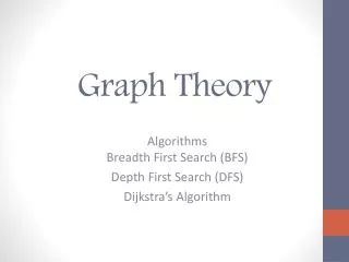
※ Many graph algorithms require a systematic method of visiting the vertices of a graph depth-first search (DFS, 深先搜尋) bread-first search (BFS, 廣先搜尋)
v2 1 v1 v6 v5 v4 v3 v7 Depth-first search G 假設G用其adjacency list來表示,而list中,每個點的neighbor依下標由小排到大 v1 v2 v3 v4 v6 v5 v7 Step 1: visit v1
v2 1 v1 v6 2 v5 v4 v3 v7 v2 1 v1 v6 2 3 v5 v4 v3 v7 G v1 v2 v3 v4 v6 v5 v7 Step 2: visit v3 Step 3: visit v5
v2 1 v1 v6 2 3 v5 v4 v3 4 v7 5 v2 1 v1 v6 2 3 v5 v4 v3 4 v7 G v1 v2 v3 v4 v6 v5 v7 Step 4: visit v7 Step 5: visit v2
5 v2 1 v1 v6 2 3 v5 6 v4 v3 4 v7 depth-first search index 5 v2 1 v1 7 v6 2 3 v5 6 v4 v3 dfi(v5)=3 4 v7 G v1 v2 v3 v4 v6 v5 v7 Step 6: visit v4 Step 7: visit v6 DFS forest
DFS forest G F v5 v5 v13 v13 v8 v8 v2 v2 v12 v7 v12 v7 v6 v6 v1 v1 v10 v10 v15 v15 v14 v14 v4 v4 v9 v9 v3 v3 v11 v11 3 12 9 2 5 4 11 10 1 7 8 15 14 13 6
rooted forest DFS forest 1 v1 6 v3 G F F’ 3 v5 12 v13 v5 v2 2 v13 7 8 v8 v4 v8 v2 v9 v2 9 2 5 v12 v7 4 v12 v7 v6 v5 v6 3 11 10 v1 v1 4 5 v10 v10 1 v7 9 v6 v12 v15 v15 7 v14 v14 8 15 v4 v10 v4 v9 v9 10 14 v3 v8 v11 v3 v11 13 v11 13 11 6 14 15 v14 v15 12 v13 back edge
Algorithm 3.1 (DFS algorithm) 1. dfi(v) 0 vV(G) 2. i 1 /* 用來assign 點的 dfi值 */ 3. S /* 用來存放 DFS forest 的所有 arc */ 4. If dfi(r) 0 r V(G), then output S and stop; otherwise, let r be the first vertex s. t. dfi(r) = 0 and let w r. /* r是這個 component 的tree 的 root */ 5. dfi(w) i 6. i i + 1 7. (search) 7.1. If dfi(v) = 0 for some v in the adjacency list of w, then continue; otherwise, go to Step 7.4. 7.2 S S∪ {(w, v)} and assign parent(v) w. 7.3 w v and return to Step 5. 7.4 If w r, thenw parent(w) and return to Step7.1; otherwise, return to Step 4.
※ Time complexity of Alg. 3.1: O(max{p, q}) Thm 3.8. Every back edge e of a graph G joins an ancestor and a descendant. In particular, if e = uv and u is visited before v in the depth-first search of G, then v is a descendant of u.
Exercise1. For the graph G shown below, find thedepth-first search forest. (不必為rooted形式) G v5 v12 v3 v9 v4 v2 v1 v11 v7 v6 v8 v10
Outline 3.1 Properties of trees 3.2 Rooted trees 3.3 Depth-first search 3.5 Breadth-first search 3.6 The minimum spanning tree problem
3.5 Breadth-first Search BFS: visit過點v後,先visit完點v的每個neighbor, 將之存入queue中,再從queue中選取第一個 點visit,依此類推
v5 v13 G v8 v2 v12 v7 v6 v1 v10 v15 v14 v4 v9 v3 v11 Step 1: visit v1 Queue 1 v1 v1
v5 v13 G v8 v2 v12 v7 v6 v1 v10 v15 v14 v4 v9 v3 v11 7 v12 5 v6 2 v2 1 v1 6 v9 4 v4 3 v3 Step 2: visit neighbors of v1 Queue v1 v2 v3 v4 v6 v9 v12
v5 v13 G v8 v2 v12 v7 v6 v1 v10 v15 v14 v4 v9 v3 v11 8 v5 7 v12 2 v2 v1 v2 v3 v4 v6 v9 v12 5 v6 1 v1 6 v9 4 v4 3 v3 Step 3: visit neighbors of v2 Queue v5
v5 v13 G v8 v2 v12 v7 v6 v1 v10 v15 v14 v4 v9 v3 v11 8 v5 7 v12 2 v2 5 v6 9 v7 1 v1 6 v9 4 v4 3 v3 Step 4: visit v7 Queue v7
v5 v13 G v8 v2 v12 v7 v6 v1 v10 v15 v14 v4 v9 v3 v11 8 v5 11 v13 7 v12 2 v2 5 v6 9 v7 1 v1 10 v10 6 v9 4 v4 3 v3 Step 5: visit neighbors ofv7 Queue v7 v10 v13
v5 v13 G v8 v2 v12 v7 v6 v1 v10 v15 v14 v4 v9 v3 v11 8 v5 11 v13 v8 12 9 v7 7 v12 2 v2 5 v6 10 v10 1 v1 6 v9 4 v4 15 13 14 3 v3 v15 v11 v14 Step 6: visit neighbors ofv10 Queue v10 v13 v8 v11 v14 v15 所有點皆已visit BFS forest
Exercise2. For the graph G shown below, find thebreadth-first search forest. G v5 v12 v3 v9 v4 v2 v1 v11 v7 v6 v8 v10
Outline 3.1 Properties of trees 3.2 Rooted trees 3.3 Depth-first search 3.5 Breadth-first search 3.6 The minimum spanning tree problem
3.6 The minimum spanning tree problem Definition: (1) weighted graph:graph 中每個 edge 上有 weight (2) weightw(H) of a subgraphH of a weighted graph: the sum of the weights of the edges of H The Minimum Spanning Tree Problem : Find a minimum spanning tree in all connected weighted graph.
Algorithm 3.3 (Kruskal’s Algorithm) 1. S ← . 2. Let e be an edge of minimum weight such that eS and <S∪{e}> is acyclic, and let S ← S∪{e}. 3. If |S| = p – 1, then output S; otherwise, return to Step 2. 建議:在 step2 執行前先將 G 的 edge 依 weight 由小至大排列 O(p2)
y FIGURE 3-18 2 5 G 5 x 3 4 6 w 2 2 1 v u y y 2 x x w w 1 v 1 v u u Sort the edges of G: uv, xy, vw, uw, ux, vx, vy, uy, wx Constructing the tree by Kruskal algorithm Step 2 Step 1 S={uv} S={uv, xy}
y FIGURE 3-18 2 5 G 5 x 3 4 6 w 2 2 y y 1 v u 2 2 x x 3 w w 2 2 1 v 1 v u u Sort the edges of G: uv, xy, vw, uw, ux, vx, vy, uy, wx Constructing the tree Step 3 Step 4 |S|=p-1 stop! S={uv, xy, vw} S={uv, xy, vw, ux}
Theorem 3.12. Kruskal’s algorithm produces a minimum spanning tree in a nontrivial connected weighted graph. Pf : Let G be a nontrivial connected weighted graph of order p, and let T be a subgraph produced by Kruskal’s algorithm. Certainly, T is a spanning tree of G (and so has size p – 1), say E(T) = { e1, e2, …, ep-1 } where w(e1) w(e2) … w(ey-1). Therefore, the weight of T is
Proof of Thm 3.12 (continued): Suppose, to the contrary, that T is not a minimum spanning tree. Then, among the minimum spanning trees of G, choose one, call it H, which has a maximum number of edges in common with T. Now HT; so T has at least one edge that does not belong to H. Let ei(1 ip-1) be the first edge with ei E(T),ei E(H). {e1, e2, …, ei-1}E(H). Define G0 = H+ei. Then G0has exactly one cycle C. Since T has no cycles, there is an edge e0 of C that is not in T. e0 E(T),e0 E(H). The graph T0 = G0-e0 is also a spanning tree of G and w(T0) = w(H) + w(ei) -w(e0).