Download
1 / 25
250 likes | 381 Vues
WP5. Dynamics of supply-chain and market volatility of networks. Fernanda Strozzi Cattaneo University-LIUC Italy. WP5: Tasks overview. Coupling models Task5.5. EWDS of Blackouts T5.4. Electricity price Model T5.1. Interaction Risk T5.6. Electric power Model T5.1.

E N D
WP5 Dynamics of supply-chain and market volatility of networks Fernanda Strozzi Cattaneo University-LIUC Italy
WP5: Tasks overview Coupling models Task5.5 EWDS of Blackouts T5.4 Electricity price Model T5.1 Interaction Risk T5.6 Electric power Model T5.1 Supply chain Model T5.1, T5.5 Correlation(T5.2) Analysis(T5.3) Energy spot prices Volatility Blackouts Volatility Red=works to be presented
D5.3 (M24) Correlation analysis between electricity prices and faults in electricity grid in the Nordic countries Contents • Data provision • Data treatment • Correlation analysis: • Linear correlation coefficient • Cross Correlation function • Cross Recurrence Plots • Principal Component Analysis • Conclusions
Data provision • Monthly Disturbances • Monthly Total Consumption http://www.nordel.org • Monthly Electricity prices http://www.nordpool.com in Denmark, Finland, Norway and Sweden from January 2000 until December 2006
Data provision • Nordel is the collaboration organisation of the Transmission System Operators (TSOs) ( Denmark, Finland, Iceland, Norway and Sweden). • Nord Pool isthe Nordic Power Exchange Market Norway(1993), Sweden(1996), Finland (1997), W Denmark (1999), E Denmark (2000), Kontek (2005)
Data provision • Nordel annual report: Disturbance is an outage, forced or unintended disconnection or failed reconnection as a results of faults in the power grid • A disturbance may consist of a single fault but it can also contain many faults, typically consisting of an initial fault followed by some secondary faults. • The grid considered is the 100-400kV network
Data treatment Disturbances Electricity prices Total Consumption Denmark(*), Finland(:), Norway(.-) and Sweden(-).
Data treatment Detrended data Trends Volatilities First differences
Data treatment W=3, s=3 W=3, s=1
Linear Correlation Coefficient The linear Correlation Coefficient r between x(i) and y(i) for i=1..N with mean mx and my Correlation matrix. w=1, s=1, yellow if |r|>0.7071 (r2>0.5) confidence level of 95%
Linear Correlation Coefficient r values between Std (for VS, VD, VT) and the mean (for the others time series), |r|>0.7071 (r2>0.5), confidence level of 95%
Cross Correlation Function w=2,s=1
Cross Recurrence plot, (Marwan, 2007) CRP is a bivariate extension of RP and is a tool to analyse the dependencies between two different time systems by comparing their states (Marvan and Kurths, 2002). It can be considered as a generalization of the linear cross-correlation function (Marwan et al. 2007). where i=1, …, n, j=1, …mthe CRP matrix is defined by x(t) y(t) t t time for y(t) x(t) y(t) no embedding t time for x(t)
Cross Recurrence plot quantification % Laminarity % Determinism % Recurrence Lines diagonally oriented They represent segments of both trajectories running parallel for some time. Frequency and length of these lines are related to the similarity between the two dynamical systems not always detected by cross correlation function. One trajectory main black diagonal (LOI) If the values of the second trajectory are modified LOI becomes LOS
Cross Recurrence plot quantification: Line Of Synchronization (LOS) t=[-2:0.01:2] e=0.01
LOS calculation for electricity prices, disturbances and Total Consumption w=2,s=1, e=0.5 Sfd Tfd D D Q=80.40 Q=64.32
LOS Algorithm 1. Find the recurrence point next to the origin 2. Find the next point by looking for recurrence points in a squared window of size w=2, If the edge of the window find a recurrence point we go to step 3, else we iteratively increase the size of the window. 3. If there are subsequent recurrence points in y-direction (x-direction), the size w of the window is iteratively increased in y-direction (x-direction) until a predefined size or until no new recurrent points are met. When a new recurrence point is found we return to step 2 LOS Quality Nt is the number of targeted points Ng the number of gap points. The larger is Q the better is LOS
LOS calculation in CRP between Disturbances and the other time series. Only the CRP with at least a part of the LOS parallel to the main diagonal is considered.
Principal Component Analysis Principal Component Analysis how many independent variables Principal Factor Models Which are the independent variables and how we have to use them to build the model
Principal Component Analysis • The data have very different mean and variancesCorrelation matrix • Eigenvectors loadings • Corresponding eigenvalues • Percent ofvariance explained on that direction = 100*eigenvalue/sum(eigenvalues); • Percent of variance • Cumulative sum of variance explained
Loadings for w=1, s=1 Principal Component Analysis PC1 PC2 PC3 PC4 PC5 PC6 PC7 PC8 PC9 PC10 PC11 PC12 0.1801 -0.4014 -0.2349 -0.4308 0.0655 -0.2196 -0.2880 -0.6285 0.1153 -0.1032 0.1062 0.0023 -0.3934 -0.1531 0.2379 0.0802 -0.3920 -0.1733 -0.1521 0.1371 0.6040 -0.2497 0.3226 0.0436 0.2872 0.0083 0.1344 -0.2054 0.6711 0.2206 0.0899 0.2632 0.4220 -0.0910 0.3051 0.0378 0.1018 -0.4453 -0.3041 -0.3593 -0.1610 -0.1850 -0.0466 0.6879 -0.0987 0.1073 -0.1129 -0.0156 -0.2924 -0.1836 0.3101 -0.1076 0.1262 0.5012 -0.6616 0.0590 -0.1768 0.1009 -0.1439 -0.0518 0.1527 -0.0640 0.2032 0.4514 0.3460 -0.6499 -0.3977 0.1075 -0.0781 0.0744 -0.0624 -0.0133 0.2213 -0.4827 0.0824 0.3576 -0.0895 0.2244 0.1905 -0.1379 0.3781 0.5055 -0.2666 0.0098 -0.3963 -0.2527 0.1831 -0.1117 0.3116 -0.1412 0.3549 -0.0538 0.0358 -0.3832 -0.5822 0.0093 0.2760 0.0306 0.5399 -0.2630 -0.1996 -0.1090 0.1178 -0.0161 -0.0529 0.0168 -0.0135 -0.7023 0.2610 -0.4511 0.0570 0.3734 -0.0783 0.2393 0.0953 0.0227 -0.3546 -0.5614 0.2681 -0.0044 -0.4144 -0.2761 0.1856 -0.0793 0.1824 -0.1403 0.3181 -0.0775 -0.3328 0.4165 0.5145 0.0476 0.2985 0.0421 0.5203 -0.2574 -0.2139 -0.0787 0.0375 -0.0069 -0.1150 0.0149 -0.0860 0.7056 S D T Sdt Ddt Tdt Sfd Dfd Tfd VS VD VT
Conclusions • Linear Correlation Coefficient: • For near all the windows w and time shifts s we found a • high linear correlation between D and T or their modified versions. • Exception w=1, s=1. • For w=12 s=12 a new correlation appears between VD, Sdt(0.8138) Cross Recurrence Plot (LOS): We can detect windows and shifts to increase linear correlation: D-S -0.26920.6304; D-Sfd 0.0702 0.5466 Principal Component Analysis: 2-3 variables at least 50% variance explained More than 3 variables at least 90% variance explained
LIUC Colaborations • Qeen Mary (Physica A) • JRC (Physica A, Physica D) • COLB (under discussion) • MASA (defined) LIUC Gender Action 2 female PhD students started to work on: • Models of Supply Chain • Ranking Risk in Supply Chain 1 female student for the final project
Conferences DISSEMINATION 1_ Analysis of complex systems by means of mathematical and simulation methods (Noè, Rossi) . International Conference on applied simulation and modeling, Corfù (June 2008) 2_ Quantifying and ranking risks. IPMA world congress Rome 9-11 Nov 2008. Colicchia, Sivonen, Noè, Strozzi. 3_Application of RQA to Financial Time Series, F. Strozzi, J.M. Zaldivar, J. Zbilut, Second International workshop on Recurrence Plot, Siena, 10-12 September 2007. Reports -Application of non-linear time series analysis techniques to the Nordic spot electricity market F. Strozzi, E.Gutiérrez, C. Noè, T. Rossi, M.Serati and J.M.Zaldívar. LIUC Paper 200, october 2007 -Deliverables D5.1, D5.2 Papers 1_Time series analysis and long range correlations of Nordic spot electricity market data, H.Erzgraber, F. Strozzi, J.M. Zaldivar, H.Touchette, E. Gutierrez, D.K.Arrowsmith, submitted to Physica A 2_ Measuring volatility in the Nordic spot electricity market using Recurrence Quantification Analysis. F. Strozzi, E.Gutiérrez, C. Noè, T. Rossi, M.Serati and J.M. Zaldívar . Accepted in EPJ Special Topics. 3_ A supply chain as a serie of filter or amplificators of the bullwhip effect . Caloiero, G., Strozzi, F., Zaldívar, J.M., 2007. International Journal of Production Economics (Accepted). 4_Control and on-line optimization of one level supply chain, F. Strozzi, C.Noè, J.M. Zaldivar, submitted to IJPE, 2008