Download

1 / 106
1.08k likes | 1.36k Vues
Perspective of supply chain optimization. Tokyo University of Marine Science and Technology Mikio Kubo. Agenda. Supply Chain and Analytic IT Mathematical Programming Solver Gurobi with Python language Constrained Programming Solver SCOP Scheduling Solver OptSeq. What’s the Supply Chain?.

E N D
Perspective of supply chain optimization Tokyo University of Marine Science and Technology Mikio Kubo
Agenda • Supply Chain and Analytic IT • Mathematical Programming Solver Gurobi with Python language • Constrained Programming Solver SCOP • Scheduling Solver OptSeq
What’s the Supply Chain? IT(Information Technology)+Logistics=Supply Chain
Vehicle Routing/Scheduling Logistics Network Design Safety Stock Allocation Forecasting Revenue Management Lot-Sizing Scheduling
Logistic System, Transactional IT, Analytic IT Analytic ITModel+Algorithm= Decision Support System brain Transactional ITPOS, ERP, MRP, DRP…Automatic Information Flow nerve Logistic System=Truck, Ship, Plant, Product, Machine, … muscle
Levels of Decision Making Strategic Level A year to several years; long-term decision making Analytic IT Tactical Level A week to several months; mid-term decision making Operational Level Transactional IT Real time to several days; short-term decision making
Models in Analytic IT Supplier Plant DC Retailer Logistics Network Design Strategic Multi-period Logistics Network Design Inventory Safety stock allocation Inventory policy optimization Production Lot-sizing Scheduling Transportation Delivery Vehicle Routing Tactical Operational
How to Solve Real SC Optimization Problems Quickly • Mixed Integer Programming (MIP) SolverGurobi =>Logistics Network Design, Lot-Sizing • Constraint Programming (CP) Solver SCOP =>Lot-Sizing, Staff Scheduling • Scheduling Solver OptSeq =>Scheduling • Vehicle Routing Solver • Inventory Policy Optimization Solver ... using Python Language
Why Python? • We can do anything by importing some modules • Optimization import gurobipy (MIP)import SCOP (CP) • Draw graphsimport networkX • Also fly! import antigravity ? http://xkcd.com/353/
What’s Gurobi? MIP solver Developed by: Zonghao Gu, Edward Rothberg,Robert Bixby Free academic license
Introduction to Gurobi (1) • Create a model objectmodel = Model("Wine Blending")
Introduction to Gurobi (2) • Add variable objectsx1 = model.addVar(name="x1")x2 = model.addVar(name="x2")x3 = model.addVar(name="x3") • Model update (needed before adding constraints; lazy update!)model.update()
Introduction to Gurobi (3) • Set the objectivemodel.setObjective(15*x1 + 18*x2 + 30*x3, GRB.MAXIMIZE) • Add constraints model.addConstr(2*x1 + x2 + x3 <= 60)model.addConstr(x1 + 2*x2 + x3 <= 60)model.addConstr(x3 <= 30) • Optimizemodel.optimize()
Mr. Python is too lazy. His room is always mess. He asked to the God of Python. “How can I tide up my toys?”
The God replied from the heaven. “Use the list. The charm is “Abracadabra [ ].” Mr. Python said “L=[ ].” What a miracle! Some boxes were fallen from the heaven. The God said. “Tide up the toys using these boxes.”
OK. Everything is packed into the list. To pick up “Teddy”, just say “L[3].”
To sort the toys in alphabetical order, just say “L.sort().” Note that L is a list object and sort() is a function defined in the object called “method.”
Modeling with Lists • Add variable objects into listx=[] for i in range(3): var=model.addVar(name=“x[%s]”%i) x.append(var) • Add constraint “x1 + x2 + x3 <= 2”model.addConstr( sum(x) <= 2 ) or model.addConstr( quicksum(x) <= 2 )
Mr. Python is impatient, too. He complained to the God. “I’d like to pick my toys immediately.” The God replied from the heaven again. “Use the dictionary. The charm is “Abracadabra {}.”
Using lists and dictionaries, Mr. Python could manage his toys efficiently and lived happily ever after.
Modeling with Dictionaries • Dictionary that maps keys (“Dry”, “Medium”, “Sweet”) to variable objects x={} x[“Dry”]= model.addVar(name=“Dry”) x[“Medium”]= model.addVar(name=“Medium”) x[“Sweet”]= model.addVar(name=“Sweet”) • Add constraintmodel.addConstr( 2*x[“Dry”]+ x[“Medium”] +x[“Sweet”] <=30 )
Wine Blending with Dictionaries (1) Blends, Profit = multidict({"Dry":15, "Medium":18, "Sweet":30})=> Blends=["Dry", "Medium“, "Sweet“] List of Keys Profit[“Dry”]=15, Profit[“Medium”]=18, ... Grapes, Inventory = multidict({"Alfrocheiro":60, "Baga":60, "Castelao":30}) Use = { ("Alfrocheiro","Dry"):2, ("Alfrocheiro","Medium"):1, ("Alfrocheiro","Sweet"):1, ("Baga","Dry"):1, .... }
Wine Blending with Dictionaries (2) x = {} for j in Blends: x[j] = model.addVar(vtype="C", name="x[%s]"%j) model.update() model.setObjective(quicksum(Profit[j]*x[j] for j in Blends), GRB.MAXIMIZE) for i in Grapes: model.addConstr(quicksum(Use[i,j]*x[j] for j in Blends) <= Inventory[i], name="use[%s]"%i) model.optimize()
k-median problem • A facility location problem with min-sum object • Number of customers n=200, number of facilities selected from customer sites k=20 • Euclidian distance,coordinates are random
Formulation weak formulation
Python Code(1) from gurobipy import * model = Model("k-median") x, y = {}, {} # empty dictionaries Dictionary Data Structure Value “127cm” Variable Object Key “Hanako”, (1,2) Mapping
Python Code (2) Add variable objects “B” means binary variable or GRB.BINARY I=range(n)J=range(n)for j in J: y[j] = model.addVar(vtype="B", name="y[%s]"%j) for i in I: x[i,j] = model.addVar( vtype="B",name="x[%s,%s]"%(i,j)) model.update() Set the objective model.setObjective(quicksum(c[i,j]*x[i,j] for i in I for j in J))
Python Code (3) for i in I: model.addConstr(quicksum(x[i,j] for j in J) = = 1, "Assign[%s]"%i) for j in J: model.addConstr(x[i,j] <= y[j], "Strong[%s,%s]"%(i,j))model.addConstr(quicksum(y[j] for j in J) = = k, "k_median")
Weak formulation (result)n=200,k=20 Optimize a model with 401 Rows, 40200 Columns and 80400 NonZeros … Explored 1445 nodes (63581 simplex iterations) in 67.08 seconds Thread count was 2 (of 2 available processors) Optimal solution found (tolerance 1.00e-04) Best objective 1.0180195861e+01, best bound 1.0179189780e+01, gap 0.0099% Opt.value= 10.1801958607
Strong formulation (result) Optimize a model with 40401 Rows, 40200 Columns and 160400 NonZeros … Explored 0 nodes (1697 simplex iterations) in 3.33 seconds(No branching!) Thread count was 2 (of 2 available processors) Optimal solution found (tolerance 1.00e-04) Best objective 1.0180195861e+01, best bound 1.0180195861e+01, gap 0.0% Opt.value= 10.1801958607
k-center problem • A facility location problem with min-max object • 100 customers,10 facilities k-center (n=30,k=3) k-median (n=30,k=3)
k-Covering Problem # of uncovered customers =1 if customer is not covered parameter that is =1 if distance is less than or equal to θ
k-Covering+Binary Search Upper and Lower Bounds UB, LB while UB – LB >ε: θ= (UB+LB)/2 if opt. val. of k-covering is 0 then UB = θ else LB = θ
Traveling salesman problem • Find a minimum cost (distance) Hamiltonian circuit • World record 85,900 nodes (symmetric instance) -> We try to solve asymmetric ones.
Upper and lower bounds(80 nodes,Euclid TSP) Non-lifted MTZ constraints -> Out of memory after running 1 day
Result Optimize a model with 6480 Rows, 6400 Columns and 37762 NonZeros … Cutting planes: Gomory: 62 Implied bound: 470 MIR: 299 Zero half: 34 Explored 125799 nodes (2799697 simplex iterations) in 359.01 seconds Optimal solution found (tolerance 1.00e-04) Best objective 7.4532855108e+00, best bound 7.4525704995e+00, gap 0.0096% Opt.value= 7.45328551084
Graph coloring problem • An example that has symmetric structure of solutions • Number of nodes n=40,maximum number of colors Kmax=10 • Random graph G(n,p=0.5)
Formulation Weak formulation
n=40, Kmax=10 Optimize a model with 3820 Rows, 410 Columns and 11740 NonZeros Explored 17149 nodes (3425130 simplex iterations) in 1321.63 seconds
Improvement of the formulation Avoid symmetric variables SOS: Special Ordered Set) Type 1 model.addSOS(1,list of var.s)
Avoid symmetric variables Optimize a model with 3829 Rows, 410 Columns and 11758 NonZeros Explored 4399 nodes (1013290 simplex iterations) in 384.53 seconds MIPFocus=2(priority=proving the optimality) 67secMIPFocus=3 (priority=lower bound) 70 sec.
+SOS constraints Optimize a model with 3829 Rows, 410 Columns and 11758 NonZerosExplored 109 nodes (58792 simplex iterations) in 22.02 seconds MIPFocus=2 65 sec.,MIPFocus=3 126 sec.
Fixed-K approach Number of “bad” edges If the end vertices of an edge have the same color, the edge is called bad, and the corresponding variable z is equal to 1
Fixed-K Approach +Binary Search UB, LB := Upper and lower bounds of K while UB – LB >1: K= [ (UB+LB)/2 ] [ ] : Gauss notation if obj. fun. of Fixd-K model = 0 then UB = K else LB = K
Improved Formulation Fixed-K Approach +Binary Search