SPIRE Spectrometer Data Reduction : Mapping Observations
SPIRE Spectrometer Data Reduction : Mapping Observations. Nanyao Lu NHSC / IPAC (On behalf of the SPIRE ICC). Goals. Overview of the SPIRE spectral mapping mode: AOR and the pipeline. Brief demo on using the Spectral Cube Analysis tool in HIPE: How to visualize a SPIRE spectral cube?


SPIRE Spectrometer Data Reduction : Mapping Observations
E N D
Presentation Transcript
SPIRE Spectrometer Data Reduction: Mapping Observations Nanyao Lu NHSC/IPAC (On behalf of the SPIRE ICC)
Goals • Overview of the SPIRE spectral mapping mode: AOR and the pipeline. • Brief demo on using the Spectral Cube Analysis tool in HIPE: • How to visualize a SPIRE spectral cube? • How to extract a 1-d spectrum within an aperture? • How to generate a line intensity map?
Helpful Resources at Your Fingertips • HIPE -> Help contents: • SPIRE Data Reduction Guide (SDRG): • Sect. 6. SPIRE spectroscopy mode cookbook. • Sect. 6.7. Receipes for mapping observations. • Sect. 6.10. Cube analysis. • Herschel Data Analysis Guide (DAG): • Sect. 6. Spectral analysis for cubes. • SPIRE instrument and calibration page: • SPIRE Observer’s Manual.
SPIRE FTS Observing Modes Spatial sampling using an internal jiggle mirror (BSM): Sparse (1 BSM pointing; 2 beam spacing) Intermediate (4 BSM pointings; 1 beam spacing) Full (16 BSM pointings; 1/2 beam spacing) Spectral resolution: High Res: 1.2 GHz (0.04 cm-1); R= 1290 – 370; ΔV = 230 – 800 km/s; Medium: 7.2 GHz (0.24 cm-1); R = 210 – 60. Low: 25 GHz (0.83 cm-1 ); R = 62 – 18, Telescope pointing: Single Pointing Raster (NxM) Any observation involving either BSM jiggling or telescope raster is defined as a mapping observation.
Telescope Raster Maps SSW SLW A 3x3 telescope raster with BSM in intermediate spatial sampling
Pipeline for Mapping Data Level-1 Spectra S(σ) Collection of spectra per jiggle/raster position, in units of W/(m2 Hz sr). Preprocess Cube A list of (ra, dec, spectrum) An algorithm to assign individual spectra to the adopted map pixels. The pipeline uses the Naïve algorithm. Spatial Projection Level-2 Product: Spectral Cube Regularly gridded spectral cube in units of W/(m2 Hz sr).
The Naïve Projection in the Pipeline SSW: 2x2 raster with intermediate spatial sampling The average of spectral scans from the 3 independent pointings is taken to be the spectrum for this map pixel of 19”x19” (SSW).
Coverage Map SSW coverage map in terms of spectral scans There could be holes, as a result of dead detectors. These map pixels have spectral values of NaN. Holes can be eliminated by making map pixel size larger by reprocessing the data yourself.
Remarks • By default, the outmost, vignetteddetectors are not used in cube construction. • Unlike photometer, there is only up to a few detectors within any map pixel. Thus, detector-to-detector calibration difference (i.e., flat fielding) is more important here. • Residual telescope emission (of 0.4 Jy as of HIPE 11) could be still present in the continuum of a spectral cube. • Aperture flux correction on 1-d spectrum extraction: • If you can use a large aperture (>> the FTS beam size), it is rather trivial to extract a 1-d spectrum. • If you have a point source in the map, its photometry is best done by going back to the appropriate Level-1 spectrum that centers on the target, and performing a point-source flux calibration. • For a source that is slightly extended, aperture flux corrcetion for the extracted 1-d spectrum is tricky at this point.
Demo on Spectral Cube Analysis Tool • Described in some detail in Herschel Data Analysis Guide, Chapter 6, that comes with your HIPE. • It works on 3-d data cubes of data type “SpectralSimpleCube” or “SimpleCube.” • What can you do with this tool? We demonstrate some of its capabilities: • Cube visualization and cropping. • Extract a 1-d spectrum of data type “Spectrum1d” from a spectral cube. The result can be, as you learnt in one of our previous webinars, analyzed using HIPE Spectrum Toolbox (e.g., to fit a spectral line). • Extract a 2-d spatial image of data type “SimpleImage” from a spectral cube. The result can be analyzed easily in HIPE or any existing tools outside HIPE. As an example, we will extract a CO line intensity map here.
Demo on Spectral Cube Analysis Tool • We use the following sample data: • OBSID = 1342198923 • NGC7023; HR, 2 repeats, full spatial sampling.