Download
1 / 27
300 likes | 481 Vues
SPIRE Imaging Fourier Transform Spectrometer (FTS) Pipeline Data Processing. Nanyao Lu (NHSC/IPAC). List of Topics. Overview of SPIRE (FTS) Spectrometer Overview of the FTS Pipeline. SPIRE Spectrometer.

E N D
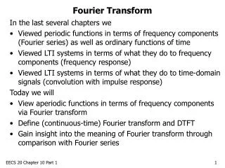
SPIRE Imaging Fourier Transform Spectrometer (FTS) Pipeline Data Processing Nanyao Lu (NHSC/IPAC)
List of Topics • Overview of SPIRE (FTS) Spectrometer • Overview of the FTS Pipeline
SPIRE Spectrometer Fourier Transform Spectrometer (FTS): The entire spectral coverage of 194-671 micron is observed in one go! (SMEC) (194-313 um) (303-671 um)
Two Bolometer Detector Arrays 303 – 671 microns 194 – 313 microns Beam = 17”- 21” Beam = 29”- 42”
Observing Modes Spectral Resolution High: 0.04 cm-1 (1.2 GHz), R=1290 – 370, e.g., line fluxes. Intermediate: 0.24 cm-1 (7.2 GHz), R = 210– 60. Low: 0.83 cm-1 (25 GHz), R = 62 – 18, e.g., dust continuum. High + Low: Both High and Low scans. Note: Data sampling at 25μm in OPD; Nyquist wave num. = 200 cm-1 Telescope Pointing Single Pointing Raster Spatial Sampling Sparse (2 beam spacing) Intermediate (1 beam spacing) Full (1/2 beam spacing; Nyquist) Spectral resolution depends on the scan length
From Interferogram to Spectrum Interferogram Source Spectrum Fourier Transform Signal (volts) Optical path difference (cm)
List of Topics • Overview of SPIRE FTS Spectrometer • Overview of the FTS Pipeline
Spectrometer Pipeline Data Flow • Level 0.5 products: • detector time lines • scan mirror time line • house keeping time lines SPIRE Common Pipeline 1. Modify Detector Timelines 2. Create Interferogram Interferograms (stored in Level 1) 3. Modify Interferogram • Level 1 products: • unmodified interfergrams • average spectrum (apodized) • average spectrum (unapodized) 4. Fourier Transform 5. Modify Spectra (V → Jy) Level 2 product: Spectral Cubes (still under development) 6. Spectral Mapping
Step 1: Modify Timelines Level 0.5 Timelines V(t) 1st Level Deglitching V(t) Cross talk matrix Remove Electrical Crosstalk V(t) Bolometer Nonlinearity Table Non-linearity Correction V(t) Bath Temperature Correction Bath temp. corr. product V(t) Clipping Correction V(t) Time constants Time-domain Phase Correction V(t) Modified Level 0.5 Timelines
Step 1: Modify Timelines Clipping Correction V(t) 1st Level Deglitching V(t) Cross talk matrix Remove Electrical Crosstalk V(t) Bolometer Nonlinearity Table Non-linearity Correction V(t) Bath Temperature Correction Bath temp. corr. product V(t) Clipping Correction V(t) Time constants Time-domain Phase Correction V(t) Modified Level 0.5 Timelines
Step 1: Modify Timelines Level 0.5 Timelines V(t) 1st Level Deglitching V(t) Cross talk matrix Remove Electrical Crosstalk V(t) Bolometer nonlinearity table Non-linearity Correction V(t) Bath Temperature Correction Bath temp. correction table V(t) Clipping Correction V(t) Time constants Time-domain Phase Correction V(t) Modified Level 0.5 Timelines
Step 2: Create Interferograms Level 0.5 Timelines V(t) Pointing P(t'') SMEC Positions x(t') V(t) Once time domain processing is complete, the detector signals and SMEC positions can be merged to create interferograms. The created “unmodified” interferograms are also stored in Level 1 in case users want to do their own interferogram-to-spectrum process. Create Interferograms Unmodified Interferograms V(x) (Stored in Level 1)
Step 2: Create Interferograms Level 0.5 Timelines V(t) Pointing P(t'') SMEC Positions x(t') V(t) Once time domain processing is complete, the detector signals and SMEC positions can be merged to create interferograms. The created “unmodified” interferograms are also stored in Level 1 in case users want to do their own interferogram-to-spectrum process. Create Interferograms Unmodified Interferograms V(x) (Stored in Level 1)
Step 3: Modify Interferograms (Level 1) Interferograms V(x) Telescope/SCAL/Beamsplitter Correction Reference background interferogram V(x) Baseline Removal V(x) 2nd Level Deglitching V(x) Phase Correction Nonlinear phase calibration table V(x) (Default apodization) Norton Beer Order-1.5 function V(x) Modified Interferogram Products (both unapodized and apodized)
Step 3: Modify Interferograms (Level 1) Interferograms V(x) Telescope/SCAL/Beamsplitter Correction Reference background interferogram V(x) Baseline Correction V(x) 2nd Level Deglitching V(x) Phase Correction Nonlinear phase V(x) (Default) Apodization Norton Beer Order-1.5 function V(x) Modified Interferogram Products
Step 4: Transform Interferograms Modified Interferograms V(x) Apply the Fourier Transform to each interferogram to create a set of spectra for each spectrometer detector. Fourier Transform SpectraV(σ)
Step 4: Transform Interferograms Modified Interferograms V(x) Apply the Fourier Transform to each interferogram to create a set of spectra for each spectrometer detector. Fourier Transform SpectraV(σ)
Step 5: Modify Spectra Spectra V(σ) Spectral Averaging V(σ) Extended-source case volt-to-Jy factors (both unapodized and apodized) Flux Conversion: V->Jy I(σ) Remove Optical Crosstalk Detector optical crosstalk matrix I(σ) Level 1 Spectrum Products Spectra are all in extended-source calibration at Level 1.
Galaxy IC 342: SLW Channel Spectra Spectra V(σ) Spectral Averaging V(σ) Flux Conversion: V->Jy Point-source case volt-to-Jy factors I(σ) Remove Optical Crosstalk Detector optical crosstalk matrix I(σ) Level 1 Spectrum Products
Galaxy IC 342: SSW Channel Spectra Spectra V(σ) Spectral Averaging V(σ) Flux Conversion: V->Jy Point-source case volt-to-Jy factors I(σ) Remove Optical Crosstalk Detector optical crosstalk matrix I(σ) Level 1 Spectrum Products
Step 6: Spatial Regridding (Level 1 to 2) Level 1 Spectra I(σ) Level 1 Spectra I(σ) Level 1 Spectra I(σ) V(t) For all observing modes but the sparse spatial sampling mode, for which only a point-source spectrum is given at Level 2. SpatialRegridding Level 2 Spectral Cube I(σ) (Under development)
Caveats and Remarks • Noise doesn’t average down as 1/sqrt(n) after about n = 25 repeats as a result of some systematic fringes. • Flux calibration is accurate to 10-20% for SSW, ~30% for SLW. • The background subtraction still uncertain below 25 cm-1 in SLW. So the continuum level could be off significantly there. However, line calibration Is not affected. • Extended-source flux calibration provided for all detector channels in all observing modes. Additional point-source calibration is provided only for the central detectors (SSWD4 & SLWC3) in the sparse observing mode. • Lines are usually unresolved, but have side lobes following a SINC function. A SINC function fit is required for total flux.
Reprocess your FTS Observations • You probably want to use data processed with the latest calibration files. • A modified HIPE 4 pipeline script is available at ~/scripts_readonly/SPIRE/spec/SPIRE_spec_SOF1_pipeline_hipe4_modified.py, which you can use to reprocess your data with any of the following options: • Use the latest calibration files (i.e., spire_cal_4_0). • Only process the central detectors (to speed up data processing & to avoid overloading your computer memory). • Using a user-supplied interferogram for telescope/sky background subtraction.
Final Spectra are great! SPIRE FTS SOF1 Pipeline and Calibration Files Trevor Fulton 25
You can play with FTS spectrum of Mrk 231 SPIRE FTS SOF1 Pipeline and Calibration Files Trevor Fulton 26 (Van der Werf etal 2010)
You can play with FTS spectrum of Mrk 231 SPIRE FTS SOF1 Pipeline and Calibration Files Trevor Fulton 27 There are 3 files in ~/scripts_readonly/spire/spec: >>> Copy the following 2 files fro there to your home directory: SPIRE_spec_SOF1_pipeline_hipe4_modified.py SCalSpecInterRef_CR_nominal_20050222_50002972_average_fourier_ALL_DETS.fits >>> Copy the following data to your ~/.hcss/lstore/ and then untar it there: 50002975.tar