Fourier Transform

1. Fourier Transform

2. Mathematical Background:Complex Numbers • A complex number x is of the form: α: real part, b: imaginary part • Addition: • Multiplication:

3. Mathematical Background:Complex Numbers (cont’d) • Magnitude-Phase (i.e.,vector) representation Magnitude: Phase: φ Magnitude-Phase notation:

4. Mathematical Background:Complex Numbers (cont’d) • Multiplication using magnitude-phase representation • Complex conjugate • Properties

5. Mathematical Background:Complex Numbers (cont’d) • Euler’s formula • Properties j

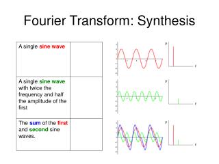
6. Mathematical Background:Sine and Cosine Functions • Periodic functions • General form of sine and cosine functions:

7. Mathematical Background:Sine and Cosine Functions Special case: A=1, b=0, α=1 π 3π/2 π/2 π 3π/2 π/2

8. Mathematical Background:Sine and Cosine Functions (cont’d) • Shifting or translating the sine function by a const b Note: cosine is a shifted sine function:

9. Mathematical Background:Sine and Cosine Functions (cont’d) • Changing the amplitude A

10. Mathematical Background:Sine and Cosine Functions (cont’d) • Changing the period T=2π/|α| consider A=1, b=0: y=cos(αt) α =4 period 2π/4=π/2 shorter period higher frequency (i.e., oscillates faster) Frequency is defined as f=1/T Alternative notation: cos(αt)=cos(2πt/T)=cos(2πft)

11. Basis Functions • Given a vector space of functions, S, then if any f(t) ϵ S can be expressed as the set of functions φk(t) are called the expansion set of S. • If the expansion is unique, the set φk(t) is a basis.

12. Image Transforms • Many times, image processing tasks are best performed in a domain other than the spatial domain. • Key steps: (1) Transform the image (2) Carry the task(s) in the transformed domain. (3) Apply inverse transform to return to the spatial domain.

13. Transformation Kernels forward transformation kernel • Forward Transformation • Inverse Transformation inverse transformation kernel

14. Kernel Properties • A kernel is said to be separable if: • A kernel is said to be symmetric if:

15. Notation • Continuous Fourier Transform (FT) • Discrete Fourier Transform (DFT) • Fast Fourier Transform (FFT)

16. Fourier Series Theorem • Any periodic function f(t) can be expressed as a weighted sum (infinite) of sine and cosine functions of varying frequency: is called the “fundamental frequency”

17. Fourier Series (cont’d) α1 α2 α3

18. Continuous Fourier Transform (FT) • Transforms a signal (i.e., function) from the spatial (x) domain to the frequency (u) domain. where

19. Why is FT Useful? • Easier to remove undesirable frequencies. • Faster perform certain operations in the frequency domain than in the spatial domain.

20. Example: Removing undesirable frequencies frequencies noisy signal remove high frequencies reconstructed signal To remove certain frequencies, set their corresponding F(u) coefficients to zero!

21. How do frequencies show up in an image? • Low frequencies correspond to slowly varying information (e.g., continuous surface). • High frequencies correspond to quickly varying information (e.g., edges) Original Image Low-passed

22. Example of noise reduction using FT Input image Spectrum Band-pass filter Output image

23. Frequency Filtering Steps 1. Take the FT of f(x): 2. Remove undesired frequencies: 3. Convert back to a signal: We’ll talk more about these steps later .....

24. Definitions • F(u) is a complex function: • Magnitude of FT (spectrum): • Phase of FT: • Magnitude-Phase representation: • Power of f(x): P(u)=|F(u)|2=

25. Extending FT in 2D • Forward FT • Inverse FT

26. Example: 2D rectangle function • FT of 2D rectangle function 2D sinc()

27. Discrete Fourier Transform (DFT) (cont’d) • Forward DFT • Inverse DFT 1/NΔx

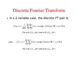
28. Extending DFT to 2D • Assume that f(x,y) is M x N. • Forward DFT • Inverse DFT:

29. Extending DFT to 2D (cont’d) • Special case: f(x,y) is N x N. • Forward DFT • Inverse DFT u,v = 0,1,2, …, N-1 x,y = 0,1,2, …, N-1

30. Extending DFT to 2D (cont’d) 2D cos/sin functions

31. Visualizing DFT • Typically, we visualize |F(u,v)| • The dynamic range of |F(u,v)| is typically very large • Apply streching: (c is const) |D(u,v)| |F(u,v)| original image before stretching after stretching

32. DFT Properties: (1) Separability • The 2D DFT can be computed using 1D transforms only: Forward DFT: kernel is separable:

33. DFT Properties: (1) Separability (cont’d) • Rewrite F(u,v) as follows: • Let’s set: • Then:

34. ) DFT Properties: (1) Separability (cont’d) • How can we compute F(x,v)? • How can we compute F(u,v)? N x DFT of rows of f(x,y) DFT of cols of F(x,v)

35. DFT Properties: (1) Separability (cont’d)

36. DFT Properties: (2) Periodicity • The DFT and its inverse are periodic with period N

37. f(x,y) F(u,v) ) N DFT Properties: (3) Translation • Translation in spatial domain: • Translation in frequency domain:

38. DFT Properties: (3) Translation (cont’d) • Warning: to show a full period, we need to translate the origin of the transform at u=N/2 (or at (N/2,N/2) in 2D) |F(u)| |F(u-N/2)|

39. ) ) N N DFT Properties: (3) Translation (cont’d) • To move F(u,v) at (N/2, N/2), take

40. DFT Properties: (3) Translation (cont’d) no translation after translation

41. DFT Properties: (4) Rotation • Rotating f(x,y) by θ rotates F(u,v) by θ

42. DFT Properties: (5) Addition/Multiplication but …

43. DFT Properties: (6) Scale

44. DFT Properties: (7) Average value Average: F(u,v) at u=0, v=0: So:

45. DFT Properties:(8) Convolution • Convolution is a common image processing technique that changes the intensities of a pixel to reflect the intensities of the surrounding pixels. A common use of convolution is to create image filters. Using convolution, you can get popular image effects like blur, sharpen, and edge detection The convolution theorem in two dimensions is expressed by the relations :

46. Magnitude and Phase of DFT • What is more important? • Hint: use the inverse DFT to reconstruct the input image using magnitude or phase only information magnitude phase

47. Magnitude and Phase of DFT (cont’d) Reconstructed image using magnitude only (i.e., magnitude determines the strength of each component!) Reconstructed image using phase only (i.e., phase determines the phase of each component!)

48. Magnitude and Phase of DFT (cont’d)