Lecture Note 5
Lecture Note 5. Discrete Random Variables and Probability Distributions. Random Variables. A random variable is a variable that takes on numerical values determined by the outcome of a random experiment. Discrete Random Variables.

Lecture Note 5
E N D
Presentation Transcript
Lecture Note 5 Discrete Random Variables and Probability Distributions
Random Variables A random variable is a variable that takes on numerical values determined by the outcome of a random experiment.
Discrete Random Variables A random variable is discrete if it can take on no more than a countable number of values.
Discrete Random Variables(Examples) • The outcome of a roll of a die. • The number of defective items in a sample of twenty items taken from a large shipment.
Continuous Random Variables A random variable is continuous if it can take any value in an interval.
Continuous Random Variables(Examples) • Heights of students in a class • Average temperature in November • The income in a year for a family. • The amount of oil imported into the U.S. in a particular month.
Discrete Random Variables • We will study the fundamental concepts of discrete random variables, namely (1) Probability Distribution Function and (2) Cumulative Probability Function. • First, we will learn the notation of the Probability Distribution Function
Understanding the notation for the probability distribution function • Suppose you are about to roll a die. Then, the number you would get after the roll is a discrete random variable. Let X denote this random variable. • Then this random variable X can take 6 possible outcomes from S={1, 2, 3, 4, 5, 6}.
Understanding the notation for the probability distribution function, contd • Then, the probability that the random variable X takes the value 1 (i.e., the probability that you get 1 after rolling the die) is 1/6. This can be conveniently expressed using the following notation: P(1)=P(X=1)=1/6 Similarly, we have P(2)=P(X=2)=1/6 P(3)=P(X=3)=1/6 . . P(6)=P(X=6)=1/6
Understanding the notation for the probability distribution function, contd • We can generalize the notation from the previous slides to other discrete random variables. Let X be any discrete random variable which takes k possible values from S={x1, x2, …, xk} Conventionally, we use capital letter X to denotes the random variable, and small letter x to denote the possible values that X can take.
Understanding the notation for the probability distribution function, contd • Now, let x be any values from S={x1, x2, …, xk} • Then, the probability that the random variable X takes the value x can be written as: P(x)=P(X=x) This notation is what it is called “Probability Distribution Function”. The next slide re-iterates this definition.
Probability Distribution Function The probability distribution function, P(x), of a discrete random variable expresses the probability that X takes the value x, as a function of x. That is
Probability Distribution Function-Exercise 1- • Ex 1-1: Suppose you roll a die. Let X be the random variable for this experiment. Find the probability distribution function P(x) by completing the table in the Excel Sheet “Probability Distribution Function Exercise”. • Ex 1-2: Plot the probability distribution function.
Probability Distribution Function-Exercise 2- • Consider the following game. You toss a coin. If you get the heads, you receive \100. If you gets the tails, you receive nothing. • The payoff for this game is a discrete random variable. Let X denote this random variable. Find the probability distribution of this random variable by completing the table in “Probability Distribution Function Exercise”.
Required Properties of Probability Distribution Functions of Discrete Random Variables Let X be a discrete random variable with probability distribution function, P(x). Then • P(x) 0 for any value of x • The individual probabilities sum to 1; that is Where the notation indicates summation over all possible values x.
Cumulative Probability Function The cumulative probability function, F(x0), of a random variable X expresses the probability that X does not exceed the value x0, as a function of x0. That is Where the function is evaluated at all values x0
Cumulative Probability Function-Example 3- • 3-1: Let X be the random variable for a roll of a die. Find F(1), F(2), F(3), to F(6). Use the Excel sheet, `Probability distribution function exercise’. • 3-2: Plot F(x) and x.
Derived Relationship Between Probability Function and Cumulative Probability Function Let X be a random variable with probability function P(x) and cumulative probability function F(x0). Then it can be shown that Where the notation implies that summation is over all possible values x that are less than or equal to x0.
Expected Value • Expected value is a similar concept as the average. More specifically, it is the weighted average with the weight given by the probability of each outcome. • For example, consider the following game. You toss a coin. If you get the heads, you receive \100. If you get the tails, you receive nothing. • Then the expected payoff for this game is \100×(probability of getting \100) + \0×(probability of getting \0) = \50 • More formally, expected value is defined as follows: See next slide.
Expected Value The expected value, E(X), of a discrete random variable X is defined Where the notation indicates that summation extends over all possible values x. The expected value of a random variable is called its mean and is denoted x.
Understanding the notation of the expected value Let X be the random variable which takes a value in S={x1, x2,..,xk}. Then the expected value of X is computed as follows. See next slide
Expected Value Exercise-Exercise 4- • Let X be the random variable that shows the number of house purchase contracts that a real estate agent can achieve in a month. The probability distribution of X is given by the following. Compute the expected number of house purchase contracts that the real estate agent can achieve in a month.
Expected Value: Functions of Random Variables Let X be a discrete random variable with probability function P(x) and let g(X) be some function of X. Then the expected value, E[g(X)], of that function is defined as
Expected Value: Functions of Random Variables-Exercise 5- • Continue using the real estate agent example. Suppose that the monthly salary for the real estate agent is given by: g(x) =$1000+ $1500*x Ex 5-1: Find the expected monthly salary of the agent. Use the “Probability Distribution Function Exercise” Excel Sheet.
Variance and Standard Deviation Let X be a discrete random variable. The expectation of the squared deviation about the mean, (X - x)2, is called the variance, denoted 2x and is given by The standard deviation, x , is the positive square root of the variance. Often we use the Var(X) to denote the varianceand SD(X) to denote the standard deviation
Understanding the procedure to compute the variance • The table in the next slide summarizes the procedure to compute variance.
Variance and Standard Deviation-Exercise 6- • Continue using the real estate agent example. Using the table in the “Probability Distribution Function Exercises” Excel sheet, answer the following questions: Ex 6-1 Compute the variance Ex 6-2 Compute the standard deviation
Summary of Properties for Linear Function of a Random Variable Let X be a random variable with mean x , and variance 2x ; and let a and b be any constant fixed numbers. Define the random variable Y = a + bX. Then, the mean and variance of Y are and so that the standard deviation of Y is
Linear Function of a Random Variable-Exercise 7- • Continue using the example of the real estate agent from exercise 4, 5, and 6. • Suppose that the monthly salary for this agent, Y, is determined in the following method: Y=$1000+ $1500*X Ex 7-1: Compute E(Y) using the formula in the previous slide. Ex 7-2: Compute the variance and standard deviation of Y
Standardization of a Random Variable Let X be a random variable with mean X and standard deviation X. Define a new random variable Z as Then E(Z)=0 Var(Z)=1
Exercise 8 • Continue using the real estate agent example. Let X be the random variable for the possible number of contracts the agent can achieve in a month. • Standardize X using the formula in the previous slide, and verify that it has mean zero and variance 1.
Reviews of Combinatorics and Common discrete distributions • Review of Combinatorics • Number of orderings • Number of combinations • Number of sequences of x Successes in n Trials • Common discrete distributions • Bernoulli Distribution • Binomial Distribution
Stock Price Movement Example • To motivate the study of combinatorics and the discrete distributions, let us consider a simple example of a stock price movement. The example will utilize combinatorics and distributions.
Stock Price Movement Example • The price of Stock A today is $10. At the end of each month the price of the stock A either goes up by the factor of 1.2 with probability 0.4, or goes down by the factor of 0.9 with probability 0.6. • This means that, if the price of the stock goes up this month, then the price of the stock in the second month will be $10×1.2 =$12. If the price of the stock goes up this month, and goes down in the second month, the price of the stock in the third month will be $10×1.2×0.9 = $10.8.
Stock Price Movement Example, Contd • Suppose that you make the following contract with a stock broker: “You have the right to purchase a share of stock A at the price equal to $37.61 at the beginning of the 13th month. • Then, if the actual market price of stock A is higher than $37.61, you purchase the stock and immediately sell it to make a positive profit (ignoring fees associated with the contract and transaction fee). If the actual price is lower than 37.61, you do not have to exercise the right. • Then consider the following question: See next slide
Stock Price Movement Example, Contd • Question What is the probability that you make some strictly positive profit from this contract (ignoring all the fees associated with the contract and buying and selling of the share)? • Answer to this question requires tools such as combinatorics and Binomial distribution. • In the following slides, we will review combinatorics and some common distributions. After studying these concepts, we will come back to the question.
Review of Combinatorics-Number of orderings- • You have n cards numbered from 1 to n. The number of ways you can order this card is given by n!=n×(n-1) ×(n-2) ×…×3×2×1 n! reads n factorial 0! is defined to be 1.
Number of ordering example • There are 5 cards numbered from 1 to 5. What is the number of ways you can order this card?
Review of Combinatorics-Combinations- • Suppose there are n cards numbered from 1 to n. If you take x cards out of n cards, the number of possible combinations of the cards is given by Where n!=n×(n-1) ×(n-2) ×…×3×2×1 Cnx reads n choose x.
Combinations -Example- • A personnel officer has eight candidate to fill four similar positions. What is the total number of possible combinations of four candidates chosen from eight?
Review of combinatorics- sequences of x Successes in n Traials- • Consider a random trial where there are only two outcomes, “Success” or “Failure”. • Then, if you make n independent trials, the number of sequences that contains exactly x successes is equal to Cnx.
Sequences of Successes-Exercise- • Consider tossing a coin 10 times. Find the number of ways the head appears exactly 4 times.
Number of sequences-Exercise- • Suppose that the figure below is a road map of a certain area. If you start from point A and walk to point B, how many possible routes can you take? (Suppose you do not walk back.) B A
Bernouli Trial Bernouli Random Trial with success probability . This is a random experiment with two possible outcomes, “success” or “failure”, where the probabilities are given by P(Success) = P(Failure) = 1-
Bernouli Random Variable • Consider a Bernouli Trial with P(Success)= . Define a random variable X in the following way. X=1 if the Bernouli random trial turn out to be success X=0 if the Bernouli random trial turns out to be a failure. Then, X is called a Bernouli Random Variable with success probability .
Bernouli Distribution • Consider a Bernouli random variable X with success probability . Then the probability distribution function for X is called Bernouli Distribution with success probability . This is given by P(0)=(1- ) and P(1)=
Bernouli Distribution -Example- • Consider the following game. You toss a coin. If you get the heads, you receive $1. If you get the tails, you receive nothing. Let X be the random variable for the payoff of this game. • X has the Bernouli distribution with success probability 0.5.
Mean and Variance of a Bernoulli Random Variable The mean is: And the variance is: