Previous Lecture: Descriptive Statistics
Previous Lecture: Descriptive Statistics. Normal. Skewed. Long tails. Complex. This Lecture. Introduction to Biostatistics and Bioinformatics Sequence Alignment Concepts. Sequence Alignment. Stuart M. Brown, Ph.D. Center for Health Informatics and Bioinformatics NYU School of Medicine.
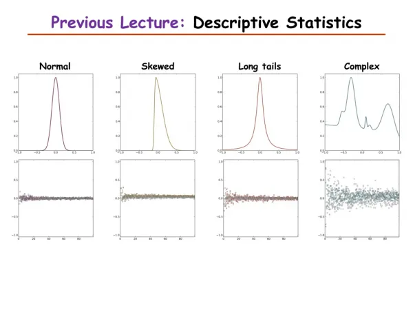

Previous Lecture: Descriptive Statistics
E N D
Presentation Transcript
Previous Lecture: Descriptive Statistics • Normal • Skewed • Long tails • Complex
This Lecture Introduction to Biostatistics and Bioinformatics Sequence Alignment Concepts
Sequence Alignment Stuart M. Brown, Ph.D. Center for Health Informatics and BioinformaticsNYU School of Medicine Slides/images/text/examples borrowed liberally from: Torgeir R. Hvidsten, Michael Schatz, Bill Pearson, Fourie Joubert, others …
Learning Objectives • Identity, similarity, homology • Analyze sequence similarity by dotplots • window/stringency • Alignment of text strings by edit distance • Scoring of aligned amino acids • Gap penalties • Global vs. local alignment • Dynamic Programming (Smith Waterman) • FASTA method
Why Compare Sequences? • Identify sequences found in lab experiments • What is this thing I just found? • Compare new genes to known ones • Compare genes from different species • information about evolution • Guess functions for entire genomes full of new gene sequences • Map sequence reads to a Reference Genome(ChIP-seq, RNA-seq, etc.)
Are there other sequences like this one? 1) Huge public databases - GenBank, Swissprot, etc. 2) “Sequence comparison is the most powerful and reliable method to determine evolutionary relationships between genes” -R. Pearson 3) Similarity searching is based on alignment 4) BLAST and FASTA provide rapid similarity searching a. rapid = approximate (heuristic) b. false + and - scores
Similarity ≠ Homology 1) 25% similarity ≥ 100 AAs is strong evidence for homology 2) Homology is an evolutionary statement which means “descent from a common ancestor” • common 3D structure • usually common function • homology is all or nothing, you cannot say "50% homologous"
Similarity is Based on Dot Plots 1) two sequences on vertical and horizontal axes of graph 2) put dots wherever there is a match 3) diagonal line is region of identity (local alignment) 4) apply a window filter - look at a group of bases, must meet % identity to get a dot
Window / Stringency Score = 11 PTHPLASKTQILPEDLASEDLTI PTHPLAGERAIGLARLAEEDFGM Filtering Score = 11 Window = 12 Stringency = 9 PTHPLASKTQILPEDLASEDLTI PTHPLAGERAIGLARLAEEDFGM Score = 7 PTHPLASKTQILPEDLASEDLTI PTHPLAGERAIGLARLAEEDFGM
Dotplot(Window = 130 / Stringency = 9) Hemoglobin-chain Hemoglobin -chain
Dotplot(Window = 18 / Stringency = 10) Hemoglobin-chain Hemoglobin -chain
How to Align Sequences? • Manually line them up and count? • an alignment program can do it for you • or a just use a text editor • Dot Plot • shows regions of similarity as diagonals GATGCCATAGAGCTGTAGTCGTACCCT <— —> CTAGAGAGC-GTAGTCAGAGTGTCTTTGAGTTCC
Percent Sequence Identity • The extent to which two nucleotide or amino acid sequences are invariant A C C T G A G – A G A C G T G – G C A G mismatch indel 70% identical
Hamming Distance • The minimum number of base changes that will convert one (ungapped) sequence into another • The Hamming distance is named after Richard Hamming, who introduced it in his fundamental paper on Hamming codes: “Error detecting and error correcting codes” (1950) Bell System Technical Journal 29 (2): 147–160. Python function hamming_distance defhamming_distance(s1, s2): #Return the Hamming distance between equal-length sequences iflen(s1) !=len(s2): raiseValueError("Undefined for sequences of unequal length") returnsum(ch1 != ch2 for ch1, ch2 inzip(s1, s2))
Hamming Dist can be unrealistic v: ATATATAT w: TATATATAHamming Dist= 8 (no gaps, no shifts) • Levenshtein (1966) introduced edit distance v = _ATATATAT w = TATATATA_ edit distance: d(v, w) = 2 Levenshtein, Vladimir I. (February 1966). "Binary codes capable of correcting deletions, insertions, and reversals". Soviet Physics Doklady10 (8): 707–710.
Gap Penalites • With unlimited gaps (no penalty), unrelated sequences can align (especially DNA) • Gap should cost much more than a mismatch • Multi-base gap should cost only a little bit more than a single base gap • Adding an additional gap near another gap should cost more (not implemented in most algorithms) • Score for a gap of length x is: -(p + σx) • p is gap open penalty • σ is gap extend penalty
GlobalvsLocalsimilarity • Globalsimilarity uses complete aligned sequences - total % matches - Needleman & Wunch algorithm 2) Local similarity looks for best internal matching region between 2 sequences - find a diagonal region on the dotplot • Smith-Waterman algorithm • BLAST and FASTA 3) dynamic programming • optimal computer solution, not approximate
Smith-Waterman Method • [Essentially finding the diagonals on the dotplot] • Basic principles of dynamic programming • - Creation of an alignment path matrix • - Stepwise calculation of score values • - Backtracking (evaluation of the optimal path)
Creation of an alignment path matrix Idea: Build up an optimal alignment using previous solutions for optimal alignments of smaller subsequences • Construct matrix F indexed by i and j (one index for each sequence) • F(i,j) is the score of the best alignment between the initial segment x1...iof x up to xi and the initial segment y1...j of y up to yj • Build F(i,j) recursively beginning with F(0,0) = 0
Creation of an alignment path matrix • If F(i-1,j-1), F(i-1,j) and F(i,j-1) are known we can calculate F(i,j) • Three possibilities: • xi and yj are aligned, F(i,j) = F(i-1,j-1) + s(xi ,yj) • xi is aligned to a gap, F(i,j) = F(i-1,j) - d • yjis aligned to a gap, F(i,j) = F(i,j-1) - d • The best score up to (i,j) will be the smallest of the three options
Choose the best option Michael Schatz Michael Schatz
Smith-Waterman is OPTIMAL but computationally slow • SW search requires computing of matrix of scores at every possible alignment position with every possible gap. • Compute task increases with the product of the lengths of two sequence to be compared (N2) • Difficult for comparison of one small sequence to a much larger one, very difficult for two large sequences, essentially impossible to search very large databases.
Scoring Similarity 1) Can only score aligned sequences 2) DNA is usually scored as identical or not 3) modified scoring for gaps - single vs. multiple base gaps (gap extension) 4) Protein AAs have varying degrees of similarity • a. # of mutations to convert one to another • b. chemical similarity • c. observed mutation frequencies 5) PAM matrix calculated from observed mutations in protein families
The 20 amino acids used in proteins have different chemical structures
ProteinScoring Systems • Amino acids have different biochemical and physical properties • that influence their relative replaceability in evolution. tiny P aliphatic C small S+S G G I A S V C N SH L D T hydrophobic Y M K E Q F W H R positive aromatic polar charged
Evolutionary Conservation: how often is one AA replaced by another in the same position in orthologous proteins?
The PAM 250 scoring matrix • Dayhoff, M, Schwartz, RM, Orcutt, BC (1978) A model of evolutionary change in proteins. in Atlas of Protein Sequence and Structure, vol 5, sup. 3, pp 345-352. M. Dayhoff ed., National Biomedical Research Foundation, Silver Spring, MD.
PAM Vs. BLOSUM PAM100 = BLOSUM90 PAM120 = BLOSUM80 PAM160 = BLOSUM60 PAM200 = BLOSUM52 PAM250 = BLOSUM45 More distant sequences • BLOSUM62 for general use • BLOSUM80 for close relations • BLOSUM45 for distant relations • PAM120 for general use • PAM60 for close relations • PAM250 for distant relations
Search with Protein, not DNA Sequences 1) 4 DNA bases vs. 20 amino acids - less chance similarity 2) can have varying degrees of similarity between different AAs - # of mutations, chemical similarity, PAM matrix 3) protein databanks are much smaller than DNA databanks
FASTA 1) A faster method to find similarities and make alignments – capable of searching many sequences (an entire database) 2) Only searches near the diagonal of the alignment matrix 3) Produces a statistic for each alignment (more on this in the next lecture)
FASTA 1) Derived from logic of the dot plot • compute best diagonals from all frames of alignment 2) Word method looks for exact matches between words in query and test sequence • hash tables (fast computer technique) • Only matches exactly identical words • DNA words are usually 6 bases • protein words are 1 or 2 amino acids • only searches for diagonals in region of word matches = faster searching
FASTA Format • simple format used by almost all programs • >header line with a [return] at end • Sequence (no specific requirements for line length, characters, etc) >URO1 uro1.seq Length: 2018 November 9, 2000 11:50 Type: N Check: 3854 .. CGCAGAAAGAGGAGGCGCTTGCCTTCAGCTTGTGGGAAATCCCGAAGATGGCCAAAGACA ACTCAACTGTTCGTTGCTTCCAGGGCCTGCTGATTTTTGGAAATGTGATTATTGGTTGTT GCGGCATTGCCCTGACTGCGGAGTGCATCTTCTTTGTATCTGACCAACACAGCCTCTACC CACTGCTTGAAGCCACCGACAACGATGACATCTATGGGGCTGCCTGGATCGGCATATTTG TGGGCATCTGCCTCTTCTGCCTGTCTGTTCTAGGCATTGTAGGCATCATGAAGTCCAGCA GGAAAATTCTTCTGGCGTATTTCATTCTGATGTTTATAGTATATGCCTTTGAAGTGGCAT CTTGTATCACAGCAGCAACACAACAAGACTTTTTCACACCCAACCTCTTCCTGAAGCAGA TGCTAGAGAGGTACCAAAACAACAGCCCTCCAAACAATGATGACCAGTGGAAAAACAATG GAGTCACCAAAACCTGGGACAGGCTCATGCTCCAGGACAATTGCTGTGGCGTAAATGGTC CATCAGACTGGCAAAAATACACATCTGCCTTCCGGACTGAGAATAATGATGCTGACTATC CCTGGCCTCGTCAATGCTGTGTTATGAACAATCTTAAAGAACCTCTCAACCTGGAGGCTT
Makes Longest Diagonal 3) after all diagonals found, tries to join diagonals by adding gaps 4) computes alignments in regions of best diagonals
FASTA Results - Alignment SCORES Init1: 1515 Initn: 1565 Opt: 1687 z-score: 1158.1 E(): 2.3e-58 >>GB_IN3:DMU09374 (2038 nt) initn: 1565 init1: 1515 opt: 1687 Z-score: 1158.1 expect(): 2.3e-58 66.2% identity in 875 nt overlap (83-957:151-1022) 60 70 80 90 100 110 u39412.gb_pr CCCTTTGTGGCCGCCATGGACAATTCCGGGAAGGAAGCGGAGGCGATGGCGCTGTTGGCC || ||| | ||||| | ||| ||||| DMU09374 AGGCGGACATAAATCCTCGACATGGGTGACAACGAACAGAAGGCGCTCCAACTGATGGCC 130 140 150 160 170 180 120 130 140 150 160 170 u39412.gb_pr GAGGCGGAGCGCAAAGTGAAGAACTCGCAGTCCTTCTTCTCTGGCCTCTTTGGAGGCTCA ||||||||| || ||| | | || ||| | || || ||||| || DMU09374 GAGGCGGAGAAGAAGTTGACCCAGCAGAAGGGCTTTCTGGGATCGCTGTTCGGAGGGTCC 190 200 210 220 230 240 180 190 200 210 220 230 u39412.gb_pr TCCAAAATAGAGGAAGCATGCGAAATCTACGCCAGAGCAGCAAACATGTTCAAAATGGCC ||| | ||||| || ||| |||| | || | |||||||| || ||| || DMU09374 AACAAGGTGGAGGACGCCATCGAGTGCTACCAGCGGGCGGGCAACATGTTTAAGATGTCC 250 260 270 280 290 300 240 250 260 270 280 290 u39412.gb_pr AAAAACTGGAGTGCTGCTGGAAACGCGTTCTGCCAGGCTGCACAGCTGCACCTGCAGCTC |||||||||| ||||| | |||||| |||| ||| || ||| || | DMU09374 AAAAACTGGACAAAGGCTGGGGAGTGCTTCTGCGAGGCGGCAACTCTACACGCGCGGGCT 310 320 330 340 350 360
Similarity Search Statistics • Searches with Needleman-Wunsch and Smith-Waterman have shown problems with simple “score” functions • Score varies with length of sequences, gap penalties, composition, protein scoring matrix, etc. • Need an unbiased method to compare alignemnts and judge if they are “significant” in a biological sense
How to score alignments? • In a large database search, the scores of good alignments differ from random alignments. • Many are random, very few good ones. • This follows an extreme value distribution, not a normal distribution. So we need to use an appropriate statistical test.
Pearson: FASTA Statistics • http://people.virginia.edu/~wrp/talk95/prot_talk12-95_4.html
Compute p-value from the extreme value distribution E is the e-value (significance score, m is your query length, n is the length of a matching database sequence, S is the score (computed from a count of matching letters with a scoring matrix and gap penalty). K is a constant computed from the database size, lambda is a constant that models the scoring system.
SimilarityStatistics • E() value is equivalent to a p value • Significant if E() < 0.05 (smaller numbers are more significant) • The E-value represents the likelihood that the observed alignment is due to chance alone. A value of 1 indicates that an alignment this good would happen by chance with any random sequence searched against this database. The official NCBI explanation of BLAST statistics by Stephen Altschul http://www.ncbi.nlm.nih.gov/BLAST/tutorial/Altschul-1.html