Descriptive Statistics
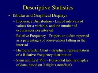
Descriptive Statistics. Statistics. Descriptive Statistic. A descriptive statistic is a numerical index that describes or summarizes some characteristic of a frequency or relative frequency distribution. (Frank & Althoen , “Statistics: Concepts and applications”, 1994)

Descriptive Statistics
E N D
Presentation Transcript
Descriptive Statistics Statistics
Descriptive Statistic A descriptive statistic is a numerical index that describes or summarizes some characteristic of a frequency or relative frequency distribution. (Frank & Althoen, “Statistics: Concepts and applications”, 1994) The discipline of quantitatively describing the main features of a collection of data or the quantitative description itself.
Descriptive Statistics • Frequency distribution table • Describe • Measures of central tendency – Mode, Median, Mean • Dispersion of distribution – Range, SD, Variance • Shape of distribution – Skewness, Kurtosis • Individuals in distributions – Percentile, Decile, Quartile • Joint distributions of data • Scatter Diagram • Correlation Coefficient • Linear Regression
Frequency Distribution Grouped Ungrouped Raw data: 42, 45, 82, 32, 91, 76, 55, 58, 55, 62, 60, … • Can be visualized using graphs and charts • Determining number of intervals • k = 1 + 3.3logN • Interval width = Range / k
Frequency Distribution Table • One-way • One variable – often used with percentage • Two-way • Two variables – shows rough relation between two variables • Etc.
Measures of Central Tendency: Mode • Mode • The value with highest frequency • Applicable to nominal scale (and higher scale) • Can be more than one value for one set of data • fx : MODE
Measures of Central Tendency: Arithmetic Mean • Considered best among the three • Sum of value divided by total frequency • Can be affected by (very) peak values • A value change of an entry also changes mean • Adding / subtracting a value from all entry changes mean for the same value • Multiply / divide all entry with a value also changes mean for the same multiplication/division with the value • Sum of the difference between each entry and mean is always zero • In case of grouped data, use sum of product of the midpoint of each interval and the frequency of that interval • fx : AVERAGE
Measures of Central Tendency: Median • Better for data with very peaked values • 5, 9, 7, 12, 89 • Ungrouped data • The value in the middle of distribution after sorting • N is odd: (N+1) / 2 • N is even: Average(N/2, N/2 +1) • Average of two middle values • fx : MEDIAN • Grouped data • See percentile
Describing Individuals in Distributions Percentile Quartile Decile Performed on data sorted in ascending order Dividing data in 100, 4, 10 parts and identify the value at the desired position
Percentile Rank • “The percentile rank of any particular score x is the percentage of observations equal to or less than x” • Divide sorted data set into 100 parts • “cent” = 100 thus “per”“cent” = /100 • Percentile rank of entry xi = 100*(cumulative frequencyi / N) • e.g. 18, 29, 31, 32, 33 • Percentile rank of 31 = 100*(3/5) = 60 • Be careful! • Percentile rank determines rank from data value • Excel uses 0.00 – 1.00 for fx: PERCENTRANK
Percentile • “The kth percentile is the x-value at or below which fall K percent of observations” • Roughly • Position of data entry at kthPercentile = k(n+1)/100 • e.g. 18, 29, 31, 32, 33 (data must first be sorted) • Percentile 80th = 80/100(5+1) = 4.8 = 5th position • Be careful! • Percentile rank determines data value from percentile • Excel uses 0.00 – 1.00 for fx: PERCENTILE
Determining Percentile in Table Determine percentile from frequency distribution table L : true lower bound of the interval containing Pr I : width of interval r : percentile in question n : number of data entry fi: accumulated frequency of the intervals below one containing Pr fr : frequency of the interval containing Pr
Determining Percentile in Table True lower bound • First, determine the interval containing the percentile in question by comparing (n x r)/100 against accumulated frequency • E.g. Percentile 37 • (188*37)/100 = 43.66 • Interval 17-24
Quartile • The kth quartile is the x-value at or below which fall K quarters of observations • Roughly • Position of data entry at kthQuartile = k(n+1)/4 • e.g. 18, 29, 31, 32, 33 (data must first be sorted) • Quartile 3th = 3/4(5+1) = 4.5 = 4th-5th position • fx: QUARTILE
Determining Quartile in Table Determine quartile from frequency distribution table L : true lower bound of the interval containing Qk I : width of interval k : quartile in question n : number of data entry fi: accumulated frequency of the intervals below one containing Qk fk: frequency of the interval containing Qk
Determining Quartile in Table True lower bound • First, determine the interval containing the quartile in question by comparing (n x k)/4 against accumulated frequency • E.g. Quartile 2 • (118*2)/4 = 59 • Interval 25-32
Decile • The kthDecile is the x-value at or below which fall K tenth of observations • Roughly • Position of data entry at kthdecile= k(n+1)/10 • e.g. 18, 29, 31, 32, 33 (data must first be sorted) • Decile 5th = 5/10(5+1) = 3rd position • Excel does not have direct decile function • Use fx: PERCENTILE with 0.1, 0.2, 0.3, … instead
Determining Decilein Table Determine decilefrom frequency distribution table L : true lower bound of the interval containing Dk I : width of interval k : decilein question n : number of data entry fi: accumulated frequency of the intervals below one containing Dk fk: frequency of the interval containing Dk
Determining Decilein Table True lower bound • First, determine the interval containing the decilein question by comparing (n x k)/10 against accumulated frequency • E.g. Decile 7 • (118*7)/10 = 83 • Interval 33-40
Dispersion of Distribution • Measures of central tendency cannot tell how data are dispersed. • Two different datasets may have a similar mean while the values are very different • 10, 20, 30, 40, 50 : mean = 30 • 5, 5, 0, 120, 20 : mean = 30 • Range • Interquartile Range and Quartile Deviation • Standard Deviation • Variance
Range • Range • Ungrouped: Max – Min (fx MAX – fx MIN) • Grouped: true highest upper bound – true lowest lower bound • True upper bound is average value between the upper bound of the interval and the (expected) lower bound of the higher interval • True lower bound is average value between the lower bound of the interval and the (expected) upper bound of the lower interval
Interquartile Range • More stable than Range as it is less affected by peak values • Quartile Deviation: QD = IR / 2 • AKA Semi-interquartile range • Use together with median
Standard Deviation & Variance • Root of the sum of difference between each entry and arithmetic mean (higher value means data are more dispersed) • OR • Standard Deviation (or SD, S.D., S) is most popular for describing dispersion N >= 30 N < 30 N >= 30 N < 30
Standard Deviation & Variance • Always SD >= 0 • SD of 0 means that all data entries are of the same value • Adding / subtracting a value from all entries does not affect SD • Multiply / divide all entries with a value m changes SD by multiplying/dividing SD with the absolute value of m • Variance (S2, SD2) is equal to SD2 • Only interested in the positive value of SD • fx : STDEV and VARA
Shape of Distribution • Skewness • 0 means there is no skewness (normal distribution) • Positive value means positive/right skewed • Negative value means negative/left skewed • fx : SKEW
Example 20 25 25 30 30 45 45 45 55 60 Positive skewed to the right
Shape of Distribution • Kurtosis • 0 means normal distribution • Positive value means very peaked (less dispersed) • Negative value means less peaked (more dispersed) • fx: KURT
Example 20 25 25 30 30 45 45 45 55 60
Correlation • Study the relationship between two variables • Does NOT infer cause and effect • Pearson Product-Moment Correlation Coefficient • Interval scale and ratio scale only • Spearman Rank Correlation Coefficient • Two ordinal-scale variables • Kendall’s Tau Rank Correlation Coefficient • Three ordinal-scale variables
Interpretation • r = 0 : two datasets have no relation • |r| <= 0.5 : the relation between two datasets is low • 0.5 < |r| < 0.8 : the relation between two datasets is mediocre • |r| >= 0.8 : the relation between two datasets is high • |r| = 1 : total relation • Can take value from -1 to 1 • Value of 1: two data sets have absolute positive relation • Value of -1: two data sets have absolute negative relation • Value of 0: two data sets have no linear relation
Joint Distribution of Data Imaginary line showing relation Imaginary line showing relation Negatively related Not related Positively related Scatter Diagram
Pearson Product-Moment Look familiar? Recall from reliability of tool? Pearson Product-Moment Correlation Coefficient Denoted as rxy or r fx: PEARSON (do not use in MS Excel earlier than 2003) fx: CORREL
Example Find the correlation between scores in mathematics exam (x) and science exam (y) of 5 students
Spearman Rank • Correlation between ranks two ordinal variables • Data are sorted and ranked • If two entries have the same value, assign the average of the rank • D = delta of ranks between data sets • N = number of pairs
Example Find correlation between ranks of theoretical exam and practice exam
Team Win Ratio Income (M$)
Kendall’s Tau Rank • Correlation between three or more ordinal variables (or sets of ranks) • Data are first sorted and ranked • N = number of pairs • D = absolute value of delta between sum of rank and mean of total rank =|r – r| • k = number of variables (or sets of ranks)
Example Find the correlation in school ranking by 3 experts
Linear Regression Describe relation between two interval-scale variables in the form of regression equation y = bx + a (Straight line) y = a + bx + cx2 (Parabola equation) y = abx(Exponential equation) x: independent variable y: dependent variable a: Y-intercept (where the line crosses Y axis) b: Slope
Simple Linear Regression • Find b then a • Then write the equation • y = bx + a • E.g. b = 31.4, a = 4.52 • y = 31.4x + 4.52
Example • Table shows the period of time each student spends reading for exam and his/her score • b = {10 (45885) – (1035)(413)} / {10 (123375) – (1035)2 • = 31395 / 162525 = 0.1932 • a = 41.3 – (0.1932) (103.5) = 21.3038 • y = 0.1932x + 21.3038 • Meaning • Spending 1 minute will increase score by 0.1932 mark • If you don’t read at all you should get 21.3038 mark
Multiple Linear Regression • More than one independent variables • Equation Y = a + b1x1 + b2x2 + b3x3… • Requirement • Normal distribution • No multicollinearity (independent variables do not depend on each other)
Multiple Linear Regression • Selecting independent variables • All Entry – when you are not sure which variable has effect • Stepwise – only use variables tested to be significant • Forward • Backward (all entry then removed insignificant variable) • Sample size must be at least 5 times of the number of variables
how much of the dependent variable can be explained by the independent variable Simple correlation Is the model good (significant)? (yes, Sig. < 0.05) b1 a b a b2


