Congestion Control
Congestion Control. Congestion: informally: “too many sources sending too much data too fast for network to handle” manifestations: lost packets (buffer overflow at routers) long delays (queuing in router buffers) a highly important problem!. Principles of Congestion Control.

Congestion Control
E N D
Presentation Transcript
Congestion: informally: “too many sources sending too much data too fast for network to handle” manifestations: lost packets (buffer overflow at routers) long delays (queuing in router buffers) a highly important problem! Principles of Congestion Control
two senders, two receivers one router, infinite buffers no retransmission Causes/costs of congestion: scenario 1
Throughput increases with load Maximum total load C (Each session C/2) Large delays when congested The load is stochastic Causes/costs of congestion: scenario 1
one router, finite buffers sender retransmission of lost packet Causes/costs of congestion: scenario 2
always: (goodput) Like to maximize goodput! “perfect” retransmission: retransmit only when loss: Actual retransmission of delayed (not lost) packet makes larger (than perfect case) for same l l l > = l l l in in in out out out Causes/costs of congestion: scenario 2
Causes/costs of congestion: scenario 2 out out out ’in ’in “costs” of congestion: • more work (retrans) for given “goodput” • unneeded retransmissions: link carries (and delivers) multiple copies of pkt
four senders multihop paths timeout/retransmit l l in in Causes/costs of congestion: scenario 3 Q:what happens as and increase ?
Causes/costs of congestion: scenario 3 Another “cost” of congestion: • when packet dropped, any “upstream” transmission capacity used for that packet was wasted!
End-end congestion control: no explicit feedback from network congestion inferred from end-system observed loss, delay approach taken by TCP Network-assisted congestion control: routers provide feedback to end systems single bit indicating congestion (SNA, DECbit, TCP/IP ECN, ATM) explicit rate sender should send at Approaches towards congestion control Two broad approaches towards congestion control:
Goals of congestion control • Throughput: • Maximize goodput • the total number of bits end-end • Fairness: • Give different sessions “equal” share. • Max-min fairness • Maximize the minimum rate session. • Single link: • Capacity R • sessions m • Each sessions: R/m
Max-min fairness • Model: Graph G(V,e) and sessions s1 … sm • For each session sia rate riis selected. • The rates are a Max-Min fair allocation: • The allocation is maximal • No ri can be simply increased • Increasing allocation rirequires reducing • Some session j • rj ≤ ri • Maximize minimum rate session.
Max-min fairness: Algorithm • Model: Graph G(V,e) and sessions s1 … sm • Algorithmic view: • For each link compute its fair share f(e). • Capacity / # session • select minimal fair share link. • Each session passing on it, allocate f(e). • Subtract the capacities and delete sessions • continue recessively. • Fluid view.
Max-min fairness • Example • Throughput versus fairness.
ABR: available bit rate: “elastic service” if sender’s path “underloaded”: sender can use available bandwidth if sender’s path congested: sender lowers rate a minimum guaranteed rate Aim: coordinate increase/decrease rate avoid loss! Case study: ATM ABR congestion control
RM (resource management) cells: sent by sender, in between data cells one out of every 32 cells. RM cells returned to sender by receiver Each router modifies the RM cell Info in RM cell set by switches “network-assisted” 2 bit info. NI bit: no increase in rate (mild congestion) CI bit: congestion indication (lower rate) Case study: ATM ABR congestion control
two-byte ER (explicit rate) field in RM cell congested switch may lower ER value in cell sender’ send rate thus minimum supportable rate on path EFCI bit in data cells: set to 1 in congested switch if data cell preceding RM cell has EFCI set, sender sets CI bit in returned RM cell Case study: ATM ABR congestion control
How does the router selects its action: selects a rate Set congestion bits Vendor dependent functionality Advantages: fast response accurate response Disadvantages: network level design Increase router tasks (load). Interoperability issues. Case study: ATM ABR congestion control
End to end feedback • Abstraction: • Alarm flag. • observable at the end stations
Simple feedback model • Every RTT receive feedback • High Congestion Decrease rate • Low congestion Increase rate • Variable rate controls the sending rate.
Multiplicative Update • Congestion: • Rate = Rate/2 • No Congestion: • Rate= Rate *2 • Performance • Fast response • Un-fair: Ratios unchanged
Additive Update • Congestion: • Rate = Rate -1 • No Congestion: • Rate= Rate +1 • Performance • Slow response • Fairness: • Divides spare BW equally • Difference remains unchanged
overflow AIMD Scheme • Additive Increase • Fairness: ratios improves • Multiplicative Decrease • Fairness: ratio unchanged • Fast response • Performance: • Congestion - Fast response • Fairness
AIMD: Two users, One link Fairness Rate of User 2 BW limit Rate of User 1
TCP Congestion Control • Closed-loop, end-to-end, window-based congestion control • Designed by Van Jacobson in late 1980s, based on the AIMD alg. of Dah-Ming Chu and Raj Jain • Works well so far: the bandwidth of the Internet has increased by more than 200,000 times • Many versions • TCP/Tahoe: this is a less optimized version • TCP/Reno: many OSs today implement Reno type congestion control • TCP/Vegas: not currently used For more details: see TCP/IP illustrated; or readhttp://lxr.linux.no/source/net/ipv4/tcp_input.c for linux implementation 29
TCP & AIMD: congestion • Dynamic window size [Van Jacobson] • Initialization: MI • Slow start • Steady state: AIMD • Congestion Avoidance • Congestion = timeout • TCP Taheo • Congestion = timeout || 3 duplicate ACK • TCP Reno & TCP new Reno • Congestion = higher latency • TCP Vegas
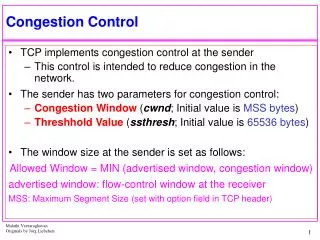
end-end control (no network assistance) transmission rate limited by congestion window size, Congwin, over segments: w * MSS throughput = Bytes/sec RTT TCP Congestion Control Congwin • w segments, each with MSS bytes sent in one RTT:
Basic structure: two “phases” slow start - MI congestion avoidance- AIMD important variables: Congwin: window size threshold: defines threshold between the slow start phase and the congestion avoidance phase “probing” for usable bandwidth: ideally: transmit as fast as possible (Congwin as large as possible) without loss increaseCongwin until congestion (loss) Congestion: decreaseCongwin, then begin probing (increasing) again TCP congestion control:
Visualization of the Two Phases Congestion avoidance threshold Congwing Slow start
exponential increase (per RTT) in window size (not so slow!) In case of timeout: Threshold=CongWin/2 Slowstart algorithm time TCP Slowstart: MI Host A Host B one segment RTT initialize: Congwin = 1 for (each segment ACKed) Congwin++ until (congestion event OR CongWin > threshold) two segments four segments
TCP Taheo Congestion Avoidance Congestion avoidance /* slowstart is over */ /* Congwin > threshold */ Until (timeout) { /* loss event */ every ACK: Congwin += 1/Congwin } threshold = Congwin/2 Congwin = 1 perform slowstart TCP Taheo
TCP Reno • Fast retransmit: • Try to avoid waiting for timeout • Fast recovery: • Try to avoid slowstart. • Single packet drop: great!
Fast Retransmit Timeout period often relatively long: long delay before resending lost packet Detect lost segments via duplicate ACKs sender often sends many segments back-to-back if segment is lost, there will likely be many duplicate ACKs If sender receives 3 ACKs for the same data, it supposes that segment after ACKed data was lost: resend segment before timer expires Packets 1 7 2 3 4 5 6 Acknowledgements (waiting seq#) 2 3 4 4 4 4 37
Fast Recovery • Fast recovery: • After retransmission do not enter slowstart. • Threshold = Congwin/2 • Congwin = 3 + Congwin/2 • Each duplicate ACK received Congwin++ • After new ACK • Congwin = Threshold • return to congestion avoidance
TCP Vegas: • Idea: track the RTT • Try to avoid packet loss • latency increases: lower rate • latency very low: increase rate • Implementation: • sample_RTT: current RTT • Base_RTT: min. over sample_RTT • Expected = Congwin / Base_RTT • Actual = number of packets sent / sample_RTT • =Expected - Actual
TCP Vegas • = Expected - Actual • Congestion Avoidance: • two parameters: and , < • If ( < ) Congwin = Congwin +1 • If ( > ) Congwin = Congwin -1 • Otherwise no change • Note: Once per RTT • Slowstart • parameter • If ( > ) then move to congestion avoidance • Timeout: same as TCP Taheo
TCP Dynamics: Rate • TCP Reno with NO Fast Retransmit or Recovery • Sending rate: Congwin*MSS / RTT • Assume fixed RTT W W/2 • Actual Sending rate: • between W*MSS / RTT and (1/2) W*MSS / RTT • Average (3/4) W*MSS / RTT
W W/2 TCP Dynamics: Loss • Loss rate (TCP Reno) • No Fast Retransmit or Recovery • Consider a cycle • Total packet sent: • about (3/8) W2 MSS/RTT = O(W2) • One packet loss • Loss Probability: p=O(1/W2) or W=O(1/p)
Q:How long does it take to receive an object from a Web server after sending a request? TCP connection establishment data transfer delay Notation, assumptions: Assume one link between client and server of rate R Assume: fixed congestion window, W segments S: MSS (bits) O: object size (bits) no retransmissions no loss, no corruption TCP latency modeling
TCP latency modeling Optimal Setting: Time = O/R Two cases to consider: • WS/R > RTT + S/R: • ACK for first segment in window returns before window’s worth of data sent • WS/R < RTT + S/R: • wait for ACK after sending window’s worth of data sent
TCP latency Modeling K:= O/WS Case 2: latency = 2RTT + O/R + (K-1)[S/R + RTT - WS/R] Case 1: latency = 2RTT + O/R
TCP Latency Modeling: Slow Start • Now suppose window grows according to slow start. • Will show that the latency of one object of size O is: where P is the number of times TCP stalls at server: - where Q is the number of times the server would stall if the object were of infinite size. - and K is the number of windows that cover the object.
TCP Latency Modeling: Slow Start (cont.) Example: O/S = 15 segments K = 4 windows Q = 2 P = min{K-1,Q} = 2 Server stalls P=2 times.