DNA Microarray Data Acquisition and Analysis - Introduction to Stanford Microarray Database
DNA Microarray Data Acquisition and Analysis - Introduction to Stanford Microarray Database. AFGC. Damares C Monte Carnegie Institution of Washington, Plant Biology Department Stanford, CA. No differential expression. Induced. Repressed. DNA Microarray Technology. AFGC. Cy5: ~650 nm.


DNA Microarray Data Acquisition and Analysis - Introduction to Stanford Microarray Database
E N D
Presentation Transcript
DNA Microarray Data Acquisition and Analysis - Introduction to Stanford Microarray Database AFGC Damares C Monte Carnegie Institution of Washington, Plant Biology Department Stanford, CA
No differential expression Induced Repressed DNA Microarray Technology AFGC Cy5: ~650 nm Cy3: ~550 nm
SMD Data Analysis • Acquisition - QC • Input/Storage/Retrieval • Analysis/Pattern Recognition • Visualization • Interpretation/Annotation • Publication/Repository Biologist
Fluorescence Intensities Extraction • To extract data from a microarray by accurately identifying the location of each of the spots. • Data extracted on: Fluorescence intensities, background intensities, fluorescence intensities ratios.
Load Images • Adjust Gain (brightness of image) and Normalization (balance between images in red and green)
Create Grids • Create new grid • Number of grids to create • Numbers of rows and columns • Spot width and height • Column and Row spacing • Resolution (Xres and Yres) • Tip spacing • Create grid
What gets flagged? Overlay Cy3 Cy5 SMD Dust speck Dust/Background/saturation/something coming into spot Doughnut Saturated on outside & in the middle doughnut Saturated in both channels Saturated in one channel Streak
Mean Intensity plots Broad distribution pattern with curved or flattened arms. Common to have gap in the center. (Crab Claw) Concentrated cluster of spots in a linear or fan pattern with clearly distinguished outliers
Median signal to background (How strong the signal is compared to background) Mean of median background (Determines how high is the background) Median signal to noise (Confidence to quantify peak signal to background) (F635Med - B635Med)/B635SD
Data Analysis Flow New Scan Gene Pix Quality Control Clustering Stanford Microarray Database - SMD Data Selection Quality Control Complete Data Table (cdt) XML Download
Comparison plot This plot can be effectively used to get a measure of the overall consistency between two duplicated or reversibly duplicated experiments. It compares the log2(RAT2N) values of the two experiments and calculates the regression line, which optimally should be close to one. Future functions will include filters and plotting of multiple experiments.
Why do we use log space? Exponential distribution of intensities Most genes at low level Very few high level Log scale approx. normal distribution ??
Frequency of intensity levelsThis plot allows the user to plot the frequency of spots within certain intensity intervals for the red and green channel respectively. It is possible to use normalized or non-normalized intensity values and linear or logarithmic scales. This graph will make it easier to determine background levels for filtering when using other analysis tools. The two examples below give a good view of what normalization does to the data.
Distribution of ratios This plot draws the distribution of the logarithm (base 2) of the red/green ratios [log2(RAT2N)]. It gives an immediate overview of the range of expression and the normality of the distribution.
Things to be Considered When Analyzing Microarray Data 1. Clones corresponding to spots with intensities of at least 350 in both channels and ratios of 2.0 / 0.5 are worth further investigation. 2. For genes of interest, check that the spot(s) is acceptable. 3. Check for consistency among replicate values. 4. Validate important results obtained from the microarray data by an independent test or method. @pilot
http://www.stat.berkeley.edu/users/terry/zarray/Html/log.htmlhttp://www.stat.berkeley.edu/users/terry/zarray/Html/log.html
Acknowledgements Shauna Somerville Katrina Ramonell Lorne Rose Bi-Huei Ho Sue Thayer Shu-Hsing Wu
Bench team Katrina Ramonell Lorne Rose Bi-Huei Ho Sue Thayer Shu-Hsing Wu Bioinformatics team David Finkelstein Jeremy Gollub Fredrik Sterky Rob Ewing Lalitha Subramanian Mira Kaloper Todd Richmond Mike Cherry AcknowledgementsShauna Somerville
http://www.stat.berkeley.edu/users/terry/zarray/Html/log.htmlhttp://www.stat.berkeley.edu/users/terry/zarray/Html/log.html