Download
1 / 33
330 likes | 425 Vues
This overview discusses improving emission inventories using direct flux measurements and modeling, with a focus on energy exchange fluxes, CO2, criteria pollutants, and VOCs. The text outlines the challenges faced at urban flux sites, presents selected results, and covers EPA STAR funded activities and measurements.

E N D
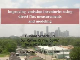
Improving emission inventories using direct flux measurements and modeling Gunnar Schade, PI Don Collins, Qi Ying (Co-PIs) Texas A&M University EPA STAR Meeting, 16 Nov. 2010
Overview • Brief Introduction • The Yellow Cab tower • challenges of an urban flux site • Selected results from previous measurements • Energy exchange fluxes • CO2 and criteria pollutants • VOCs • EPA STAR fund activities and measurements
Introduction, I • Regional Air Quality (AQ) modeling improved • uses submodels for • emissions distribution (“inventory”) • atmospheric transport and chemistry • Emissions Inventory (EI) often assumed as being known well • Ambient AQ measurements challenge some EI assumptions; inadequate? • Can the EI be improved?
Introduction, II • Past efforts of EI improvement • multivariate source apportionment using ambient AQ (concentration) data • ‘real-world’ emission measurements (tunnel studies) • AQ model studies • Our approach • micrometeorological flux measurements • top-down – bottom-up comparison • EI model AND AQ model testing
Site Description, IIland use land cover
Traffic Counts Hardy (south bound) Elysian (north bound) Quitman Road (east/west bound)
Tower Measurement Setup WS/WD aspirated T/RH Tower N PAR pyranometer w net radiation 60 m 50 m 40 m 20 m 13 m Sonic PC 20-m gradient DL Wind data (10 Hz) 3/8’’ and 1/4“ OD PFA Tubes Relaxed Eddy Accumulation Base Building GC- FID EC CO2 / H2O gradient Lag time ≈ 9 s slow: CO, NOx, O3
The challenge ‘Ordinary’ flux site Urban flux site heterogeneous land cover ill-defined footprint roughness sublayer ill-defined flux contributors high variability limited access private property undocumented activities ‘chaos’ studies attention to averages/medians • homogeneous land cover • well-defined footprint (MO theory) • well-defined flux contributors • limited variability • access to surface sites • upscaling / downscaling • targeted manipulations • process studies • attention to detail
Energy exchange fluxes, II summer winter • delayed sensible heat flux • significant latent cooling • large heat storage and release (with hysteresis)
Carbon dioxide (CO2) fluxes, I winter summer
Carbon dioxide (CO2) fluxes, II weekdays weekends
Criteria Pollutant Fluxes, I Summertime (multi-month) medians
Criteria Pollutant Fluxes, III CO-Flux ≈ ∆CO/∆CO2 x FCO2 rush-hour only
Criteria Pollutant Fluxes, IV TexAQS 2006
STAR grant activities • continued (improved) measurements (G. Schade) • criteria pollutants (ongoing) and VOCs (2011+2012) • gradient (CP, ongoing) and REA flux (VOCs, 2011+2012) • potentially EC CO fluxes (loaned instrument; 2011) • additional aerosol (flux) measurements (D. Collins) • particle number fluxes (2011+2012) • modeling (G. Schade, Qi Ying)(ongoing) • (more detailed) ground survey • GIS improvements (ongoing) • roadside measurements (2011 or 2012) • ‘undocumented’ emissions (2011)
Aerosol flux measurements, I Novel REA particle flux setup
Aerosol flux measurements, II • approx. 80 m SS tubing, laminar flow • insulated • size-dependent line loss tests • one or two instruments • Initial measurement with DMA • accumulate density measurements over 30 min • APS installed and to be used if losses not excessive • particle flux per size range per half hour
Modeling, I • GIS data • footprint models overlay • ground survey of sources • tracer release experiment
Modeling, II • Source apportionment • concentration AND flux data • CMB and PMF methods • MOBILE6 vs. MOVES • CMAQ episode modeling • alternate input based on measurements • hindcast optimization
MOBILE6 versus MOVES: Population normalized emission factors with vehicle speed (2-axle vehicles)
Roadside measurements • chemistry? depositional loss? • A&M trailer; line power from pole • subset of instruments • simultaneous traffic counts • QUIC plume modeling
Expected Results • Identify (and characterize) EI short-falls • example: missing isoprene and MACR emissions • Temporal and spatial characterization of emissions, including CP and VOCs • example: road versus non-road • Improve modeling hindcasts • characterize needed EI changes • Improve forecasts
Acknowledgements • Greater Houston Transportation Company (Yellow Cab) • Texas Air Research Center (TARC) • EPA • Bernhard Rappenglück, UH • TCEQ