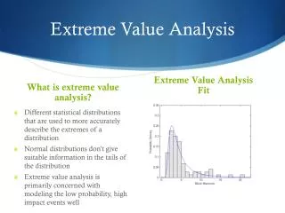
Some advanced methods in extreme value analysis
Some advanced methods in extreme value analysis. Peter Guttorp NR and UW. Outline. Nonstationary models Extreme dependence (Cooley) When a POT approach is better than a block max approach ( Wehner and Paciorek ) A Bayesian space-time model An extreme climate event. Trends.

Some advanced methods in extreme value analysis
E N D
Presentation Transcript
Some advanced methods in extreme value analysis Peter Guttorp NR and UW
Outline • Nonstationary models • Extreme dependence (Cooley) • When a POT approach is better than a block max approach (Wehner and Paciorek) • A Bayesian space-time model • An extreme climate event
Time-dependent location estimates Stockholm data (Guttorp and Xu, Environmetrics 2011)
Simple model Model Estimate -LLR Fixed μ,all -16.6 706.0 Fixed μ, early -18.1 336.8 Fixed μ, late -14.2 350.2 Early + late 687.0 Linear model in μ (-18.9,-14.0) 687.9 A linear change in mean value for annual minima seems a good model. Modal prediction for 2050: -11.5°C 2100: -10.5°C
Storm surges and wave heights Risk region Most of these data are not extreme!
Estimating H • Transform margins to Frechet; keep largest 150 obs (95th %ile)
Climate model output • Daily precip from 450 year control run of climate model (long stationary series) • Fit GEV to seasonal max
POT analysis • 99th percentile
Why are the two analyses so different? • Desert regions: large amount of lack of precipitation. GEV therefore will include many zeros, while GPD only uses data where high values are actually recorded.
Some temperature data • SMHI synoptic stations in south central Sweden, 1961-2008
Dependence between stations Common coldest day in 48 years 5 common to all 4 northern stations
Max stable processes • Independent processes Yi(x) • (e.g. space-time processes with weak temporal dependence) • A difficulty is that we cannot compute the joint distribution of more than 2-3 locations. So no likelihood.
Spatial model • where • Allows borrowing estimation strength from other sites • Can include more sites in analysis
Trend estimates Posterior probability of slope ≤ 0 is very small everywhere
What made Gudrun so destructive? • Hurricane Gudrun, Sweden, January 2005. 15 deaths, 340 000 households without power up to 4 weeks.
Consequences • 75 million cubic feet of forest fell (normal annual production) • Wind speeds up to 40 m/s • Forest damage due to large amounts of precipitation, temperatures around 0°C, high winds • Much work on multivariate extreme asymptotics needs all components to be extreme–here temperature is not. • Want (limiting) conditional distribution of wind given temperature and previous precipitation
The Heffernan-Tawn approach • Assume we can find normalizing factors a-i(yi), b-i(yi) so that • where G-i has non-degenerate margins. • Pick aji(yi) so that • and • where hji is the conditional hazard function of Yj given Yi=yi.
Asymptotic properties • Let . • Then given Yi>u, • Yi - u and Z-i are asymptotically independent as . Furthermore • Fitting using observed data; forecasting using regional model output
Some R software • ExtRemes • ismev • evlr • SpatialExtremes