Download
1 / 127
1.32k likes | 1.58k Vues
Learn about dynamic games, game trees, extensive-form representation, Nash equilibrium, and strategies in games with complete information. Dive into applications and examples to grasp key concepts.

E N D
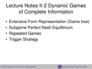
Notes modified from Yongqin Wang @ Fudan University LECTURE 3 DYNAMIC GAMES OF COMPLETE INFORMATION
Outline of dynamic games of complete information • Dynamic games of complete information • Extensive-form representation • Dynamic games of complete and perfect information • Game tree • Subgame-perfect Nash equilibrium • Backward induction • Applications • Dynamic games of complete and imperfect information • More applications • Repeated games
Entry game • An incumbent monopolist faces the possibility of entry by a challenger. • The challenger may choose to enter orstay out. • If the challenger enters, the incumbent can choose either to accommodate or tofight. • The payoffs are common knowledge. Challenger In Out Incumbent The first number is the payoff of the challenger. The second number is the payoff of the incumbent. 1, 2 A F 2, 1 0, 0
Sequential-move matching pennies Player 1 • Each of the two players has a penny. • Player 1 first chooses whether to show the Head or the Tail. • After observing player 1’s choice, player 2 chooses to show Head or Tail • Both players know the following rules: • If two pennies match (both heads or both tails) then player 2 wins player 1’s penny. • Otherwise, player 1 wins player 2’s penny. H T Player 2 Player 2 H T H T -1, 1 1, -1 1, -1 -1, 1
Dynamic (or sequential-move) games of complete information • A set of players • Who moves when and what action choices are available? • What do players know when they move? • Players’ payoffs are determined by their choices. • All these are common knowledge among the players.
Definition: extensive-form representation • The extensive-form representation of a game specifies: • the players in the game • when each player has the move • what each player can do at each of his or her opportunities to move • what each player knows at each of his or her opportunities to move • the payoff received by each player for each combination of moves that could be chosen by the players
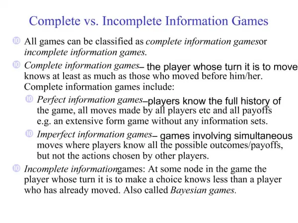
Dynamic games of complete and perfect information • Perfect information • All previous moves are observed before the next move is chosen. • A player knows Who has moved What before she makes a decision
Game tree x0 • A game tree has a set of nodes and a set of edges such that • each edge connects two nodes (these two nodes are said to be adjacent) • for any pair of nodes, there is a unique path that connects these two nodes a path from x0 to x4 a node x2 x1 x3 x4 x5 x6 x7 x8 an edge connecting nodes x1 and x5
Game tree a path from x0 to x4 x0 • A path is a sequence of distinct nodes y1, y2, y3, ..., yn-1, yn such that yi and yi+1 are adjacent, for i=1, 2, ..., n-1. We say that this path is from y1 to yn. • We can also use the sequence of edges induced by these nodes to denote the path. • The length of a path is the number of edges contained in the path. • Example 1: x0, x2, x3, x7 is a path of length 3. • Example 2: x4, x1, x0, x2, x6 is a path of length 4 x2 x1 x3 x4 x5 x6 x7 x8
Game tree x0 • There is a special node x0 called the root of the tree which is the beginning of the game • The nodes adjacent to x0 are successors of x0. The successors of x0 are x1, x2 • For any two adjacent nodes, the node that is connected to the root by a longer path is a successor of the other node. • Example 3: x7 is a successor of x3 because they are adjacent and the path from x7 to x0 is longer than the path from x3 to x0 x2 x1 x3 x4 x5 x6 x7 x8
Game tree x0 • If a node x is a successor of another node y then y is called a predecessor of x. • In a game tree, any node other than the root has a unique predecessor. • Any node that has no successor is called a terminal node which is a possible end of the game • Example 4: x4, x5, x6, x7, x8 are terminal nodes x2 x1 x3 x4 x5 x6 x7 x8
Game tree Player 1 • Any node other than a terminal node represents some player. • For a node other than a terminal node, the edges that connect it with its successors represent the actions available to the player represented by the node H T Player 2 Player 2 H T H T -1, 1 1, -1 1, -1 -1, 1
Game tree Player 1 • A path from the root to a terminal node represents a complete sequence of moves which determines the payoff at the terminal node H T Player 2 Player 2 H T H T -1, 1 1, -1 1, -1 -1, 1
Strategy • A strategy for a player is a complete plan of actions. • It specifies a feasible action for the player in every contingency in which the player might be called on to act. • What the players canpossibly play, not what they do play. • Cf: static games
Challenger’s strategies In Out Incumbent’s strategies Accommodate (if challenger plays In) Fight (if challenger plays In) Payoffs Normal-form representation Entry game
Strategy and payoff • In a game tree, a strategy for a player is represented by a set of edges. • A combination of strategies (sets of edges), one for each player, induce one path from the root to a terminal node, which determines the payoffs of all players
Sequential-move matching pennies • Player 1’s strategies • Head • Tail • Player 2’s strategies • H if player 1 plays H, H if player 1 plays T • H if player 1 plays H, T if player 1 plays T • T if player 1 plays H, H if player 1 plays T • T if player 1 plays H, T if player 1 plays T Player 2’s strategies are denoted by HH, HT, TH and TT, respectively.(n x m)
Their payoffs Normal-form representation Sequential-move matching pennies
Nash equilibrium • The set of Nash equilibria in a dynamic game of complete information is the set of Nash equilibria of its normal-form.
Nash equilibrium in a dynamic game • We can also use normal-form to represent a dynamic game • The set of Nash equilibria in a dynamic game of complete information is the set of Nash equilibria of its normal-form • How to find the Nash equilibria in a dynamic game of complete information • Construct the normal-form of the dynamic game of complete information • Find the Nash equilibria in the normal-form
Two Nash equilibria ( In, Accommodate ) ( Out, Fight ) Does the second Nash equilibrium make sense? Non-creditable threats Limitation to the normal form representation Nash equilibria in entry game
Remove nonreasonable Nash equilibrium • Subgame perfect Nash equilibrium is a refinement of Nash equilibrium • It can rule out nonreasonable Nash equilibria or non-creditable threats • We first need to define subgame
Player 1 H T Player 2 Player 2 H T H T 1, -1 1, -1 -1, 1 a subgame Subgame • A subgame of a game tree begins at a nonterminal node and includes all the nodes and edges following the nonterminal node • A subgame beginning at a nonterminal node x can be obtained as follows: • remove the edge connecting x and its predecessor • the connected part containing x is the subgame -1, 1
Player 1 C D Player 2 Player 2 2, 0 E F E F Player 1 Player 1 3, 1 3, 1 G H G H Player 1 1, 2 0, 0 1, 2 0, 0 G H 1, 2 0, 0 Subgame: example
Subgame-perfect Nash equilibrium • A Nash equilibrium of a dynamic game is subgame-perfect if the strategies of the Nash equilibrium constitute a Nash equilibrium in every subgame of the game. • Subgame-perfect Nash equilibrium is a Nash equilibrium.
Challenger Incumbent In Out A F Incumbent 1, 2 A F 2, 1 0, 0 2, 1 0, 0 Entry game • Two Nash equilibria • ( In, Accommodate ) is subgame-perfect. • ( Out, Fight ) is not subgame-perfect because it does not induce a Nash equilibrium in the subgame beginning at Incumbent. Accommodate is the Nash equilibrium in this subgame.
Find subgame perfect Nash equilibria: backward induction • Starting with those smallest subgames • Then move backward until the root is reached Challenger In Out Incumbent 1, 2 A F The first number is the payoff of the challenger. The second number is the payoff of the incumbent. 2, 1 0, 0
Player 1 C D Player 2 2, 0 E F Player 1 3, 1 G H 1, 2 0, 0 Find subgame perfect Nash equilibria: backward induction • Subgame perfect Nash equilibrium (DG, E) • Player 1 plays D, and plays G if player 2 plays E • Player 2 plays E if player 1 plays C
Existence of subgame-perfect Nash equilibrium • Every finite dynamic game of complete and perfect information has a subgame-perfect Nash equilibrium that can be found by backward induction.
Sequential bargaining (2.1.D of Gibbons) • Player 1 and 2 are bargaining over one dollar. The timing is as follows: • At the beginning of the first period, player 1 proposes to take a share s1 of the dollar, leaving 1-s1 to player 2. • Player 2 either accepts the offer or rejects the offer (in which case play continues to the second period) • At the beginning of the second period, player 2 proposes that player 1 take a share s2 of the dollar, leaving 1-s2 to player 2. • Player 1 either accepts the offer or rejects the offer (in which case play continues to the third period) • At the beginning of third period, player 1 receives a share s of the dollar, leaving 1-s for player 2, where 0<s <1. • The players are impatient. They discount the payoff by a fact , where 0< <1
Sequential bargaining (2.1.D of Gibbons) Player 1 propose an offer ( s1 , 1-s1 ) Period 1 Player 2 s1 , 1-s1 accept reject Player 2 propose an offer ( s2 , 1-s2 ) Player 1 s2 , 1-s2 Period 2 accept reject Period 3 s , 1-s
Solve sequential bargaining by backward induction • Period 2: • Player 1 accepts s2 if and only if s2 s. (We assume that each player will accept an offer if indifferent between accepting and rejecting) • Player 2 faces the following two options:(1) offers s2 = s to player 1, leaving 1-s2 = 1-s for herself at this period, or(2) offers s2 < s to player 1 (player 1 will reject it), and receives 1-s next period. Its discounted value is (1-s) • Since (1-s)<1-s, player 2 should propose an offer (s2* , 1-s2* ), where s2* = s. Player 1 will accept it.
Sequential bargaining (2.1.D of Gibbons) Player 1 propose an offer ( s1 , 1-s1 ) Period 1 Player 2 s1 , 1-s1 accept reject s , 1-s Player 2 propose an offer ( s2 , 1-s2 ) Player 1 s2 , 1-s2 Period 2 accept reject Period 3 s , 1-s
Solve sequential bargaining by backward induction • Period 1: • Player 2 accepts 1-s1 if and only if 1-s1 (1-s2*)=(1- s) or s1 1-(1-s2*), where s2* = s. • Player 1 faces the following two options:(1) offers 1-s1 = (1-s2*)=(1- s)to player 2, leaving s1 = 1-(1-s2*)=1-+s for herself at this period, or(2) offers 1-s1 < (1-s2*)to player 2 (player 2 will reject it), and receives s2* = s next period. Its discounted value is s • Since s < 1-+s, player 1 should propose an offer (s1* , 1-s1* ), where s1* = 1-+s
Player 1 H T Player 2 Player 2 H T H T -1, 1 1, -1 1, -1 -1, 1 Strategy and payoff a strategy for player 1: H • A strategy for a player is a complete plan of actions. • It specifies a feasible action for the player in every contingency in which the player might be called on to act. • It specifies what the player does at each of her nodes a strategy for player 2: H if player 1 plays H, T if player 1 plays T (written as HT) Player 1’s payoff is -1 and player 2’s payoff is 1 if player 1 plays H and player 2 plays HT
Player 1 H T Player 2 Player 2 H T H T 1, -1 1, -1 -1, 1 a subgame Subgame • A subgame of a game tree begins at a nonterminal node and includes all the nodes and edges following the nonterminal node • A subgame beginning at a nonterminal node x can be obtained as follows: • the connected part containing x is the subgame • remove the edge connecting x and its predecessor -1, 1
Existence of subgame-perfect Nash equilibrium • Every finite dynamic game of complete and perfect information has a subgame-perfect Nash equilibrium that can be found by backward induction.
Player 1 D C Player 2 Player 2 E G F H 2, 1 0, 2 3, 0 1, 3 Backward induction: illustration • Subgame-perfect Nash equilibrium (C, EH). • player 1 plays C; • player 2 plays E if player 1 plays C, plays H if player 1 plays D.
Player 2 Player 2 Player 2 H F J I G K 2, 2 1, 1 0, 1 2, 1 1, 0 1, 3 Multiple subgame-perfect Nash equilibria: illustration • Subgame-perfect Nash equilibrium (D, FHK). • player 1 plays D • player 2 plays F if player 1 plays C, plays H if player 1 plays D, plays K if player 1 plays E. Player 1 E C D
Player 2 Player 2 Player 2 H F J I G K 2, 2 1, 1 0, 1 2, 1 1, 0 1, 3 Multiple subgame-perfect Nash equilibria • Subgame-perfect Nash equilibrium (E, FHK). • player 1 plays E; • player 2 plays F if player 1 plays C, plays H if player 1 plays D, plays K if player 1 plays E. Player 1 E C D
Player 2 Player 2 Player 2 H F J I G K 2, 2 1, 1 0, 1 2, 2 1, 0 1, 3 Multiple subgame-perfect Nash equilibria • Subgame-perfect Nash equilibrium (D, FIK). • player 1 plays D; • player 2 plays F if player 1 plays C, plays I if player 1 plays D, plays K if player 1 plays E. Player 1 E C D
Stackelberg model of duopoly • A homogeneous product is produced by only two firms: firm 1 and firm 2. The quantities are denoted by q1 and q2, respectively. • The timing of this game is as follows: • Firm 1 chooses a quantity q10. • Firm 2 observes q1 and then chooses a quantity q20. • The market priced is P(Q)=a –Q, where a is a constant number and Q=q1+q2. • The cost to firm i of producing quantity qi is Ci(qi)=cqi. • Payoff functions:u1(q1, q2)=q1(a–(q1+q2)–c)u2(q1, q2)=q2(a–(q1+q2)–c)
Stackelberg model of duopoly • Find the subgame-perfect Nash equilibrium by backward induction • We first solve firm 2’s problem for any q10 to get firm 2’s best response to q1 . That is, we first solve all the subgames beginning at firm 2. • Then we solve firm 1’s problem. That is, solve the subgame beginning at firm 1
Stackelberg model of duopoly • Solve firm 2’s problem for any q10 to get firm 2’s best response to q1. • Maxu2(q1, q2)=q2(a–(q1+q2)–c)subject to 0 q2 +∞FOC: a – 2q2 – q1–c = 0 • Firm 2’s best response, • R2(q1) = (a – q1–c)/2 if q1 a–c = 0 if q1> a–cNote: Osborne used b2(q1) instead of R2(q1)
Stackelberg model of duopoly • Solve firm 1’s problem. Note firm 1 can also solve firm 2’s problem. That is, firm 1 knows firm 2’s best response to any q1. Hence, firm 1’s problem is • Max u1(q1, R2(q1))=q1(a–(q1+R2(q1))–c)subject to 0 q1 +∞That is,Max u1(q1, R2(q1))=q1(a–q1–c)/2subject to 0 q1 +∞FOC: (a – 2q1 –c)/2= 0 q1 = (a–c)/2
Stackelberg model of duopoly • Subgame-perfect Nash equilibrium • ( (a–c)/2, R2(q1) ), whereR2(q1) = (a – q1–c)/2 if q1 a–c = 0 if q1> a–c • That is, firm 1 chooses a quantity (a–c)/2, firm 2 chooses a quantity R2(q1) if firm 1 chooses a quantity q1. • The backward induction outcome is ( (a–c)/2, (a–c)/4 ). • Firm 1 chooses a quantity (a–c)/2, firm 2 chooses a quantity (a–c)/4.
Stackelberg model of duopoly • Firm 1 producesq1=(a–c)/2 and its profitq1(a–(q1+ q2)–c)=(a–c)2/8 • Firm 2 producesq2=(a–c)/4 and its profitq2(a–(q1+ q2)–c)=(a–c)2/16 • The aggregate quantity is 3(a–c)/4.
Cournot model of duopoly • Firm 1 producesq1=(a–c)/3 and its profitq1(a–(q1+ q2)–c)=(a–c)2/9 • Firm 2 producesq2=(a–c)/3 and its profitq2(a–(q1+ q2)–c)=(a–c)2/9 • The aggregate quantity is 2(a–c)/3.
Monopoly • Suppose that only one firm, a monopoly, produces the product. The monopoly solves the following problem to determine the quantity qm. • Maxqm(a–qm–c)subject to 0 qm +∞FOC: a – 2qm –c = 0 qm = (a–c)/2 • Monopoly producesqm=(a–c)/2 and its profitqm(a–qm–c)=(a–c)2/4
Discusssion • The first-mover advantage • Strategic substitutes and commitment (threat) • Stackelberg model • Strategic complements and commitment • Bertrand model (your task) • The curse of knowledge • It is a good thing for rational one-agent decision problem • Not for a person with self-control • The last leaf (O.Henry)