The Theory of the Simplex Method
250 likes | 699 Vues
The Theory of the Simplex Method. The Essence. Simplex method is an algebraic procedure However, its underlying concepts are geometric Understanding these geometric concepts helps before going into their algebraic equivalents

The Theory of the Simplex Method
E N D
Presentation Transcript
The Essence • Simplex method is an algebraic procedure • However, its underlying concepts are geometric • Understanding these geometric concepts helps before going into their algebraic equivalents • With two decision variables, the geometric concepts are easy to visualize • Should understand the generalization of these concepts to higher dimensions
Standard (Canonical) Form of an LP Model Maximize Z = c1x1 + c2x2 + … + cnxn subject to a11x1 + a12x2 + … + a1nxn≤ b1 a21x1 + a22x2 + … + a2nxn ≤ b2 … am1x1 + am2x2 + … + amnxn ≤ bm x1≥ 0, x2≥ 0, …, xn≥ 0
Extended Terminology max cx n variables s.to Ax b m inequalities x 0 n inequalities max cx n+m variables s.to Ax + Ixs = b m equations x, xs 0 n+m inequalities • Constraint boundary equation • For any constraint, obtain by replacing its , =, by = • It defines a “flat” geometric shape: hyperplane • Corner-point solution • Simultaneous solution of n constraint boundary equations ( )
Extended Terminology max cx + 0xsn+m variables s.to Ax + Ixs = b m equations x, xs 0 n+m inequalities • Indicating variables (in the augmented form)
Properties of CPF (BF) Solutions Property 1: • If there is exactly one optimal solution, then it must be a corner-point feasible solution • If there are multiple optimal solutions (and a bounded feasible region), then at least two must be adjacent corner-point feasible solutions Proof of (a) by contradiction
Properties of CPF (BF) Solutions Property 2: There are only a finite number of corner-point feasible solutions max cx n variables s.to Ax b m inequalities x 0 n inequalities CP solution is defined as the intersection of n constraint boundary equations (n+m) choose n: Upper bound on # of CPF solutions
Properties of CPF (BF) Solutions Property 3: • If a corner-point feasible solution has no adjacent CPF solution that are better, then there are no better CPF solutions elsewhere • Hence, such a CPF solution is an optimal solution (assuming LP is feasible and bounded)
Simplex in Matrix (Product) Form max cx n variables s.to Ax b m inequalities x 0 n inequalities max cx m+n variables s.to Ax + Ixs = b m equations x, xs 0 m+n inequalities Initial Tableau: ( ) XB=
Simplex in Matrix (Product) Form Intermediate iterations: • Let B denote the square matrix that contains the columns from [ A | I ] that correspond to the current set of basic variables, xB(in order) • Similarly, let cB be the vector of elements in c that correspond to xB • Then at any intermediate step, the simplex tableau is given by
Revised Simplex Method • InitializationFind an initial BFS (if one not immediately available, do Phase 1. If Phase 1 terminates with z1>0, LP is infeasible) • Optimality testCalculate cBB-1A-c for basic,and cBB-1for nonbasic variables. If all ≥ 0, stop with optimality • Iterative step • Determine the entering variable as before (steepest ascent) • Let xk be the entering variable • Determine the leaving variable as before (minimum ratio test), but now only need to calculate the coefficients of the pivot column (from B-1A or B-1) and the updated rhs (B-1b) • Let xl : the leaving variable r : the equation number of the leaving variable a’rk : coefficient of xk in rth equation (the pivot element) • Determine B-1new=E B-1old where E is I expect for rth column replaced with • Can calculate the new BFS using xB=B-1b and z=cBB-1b • Back to optimality test
Original data: Revised Simplex Example Maximize z = 2x1+ 3x2 subject to x1 + 2x2≤ 10 3x1+ x2≤ 15 x2≤ 4 x1,x2 ≥0 Maximize z = 2x1+ 3x2 subject to x1 + 2x2+s1= 10 3x1+ x2+s2 = 15 x2+s3= 4 x1,x2, s1, s2, s3 ≥ 0
Iteration 0 • Calculate row-0 coefficients: cBB-1A-c = cBB-1 = Optimal? • Entering variable is • Calculate coefficients in pivot column using B-1A or B-1 • Calculate updated rhs using B-1b, do the ratio test • Leaving variable is • Update B-1
Iteration 1 • Calculate row-0 coefficients: cBB-1A-c = cBB-1 = Optimal? • Entering variable is • Calculate coefficients in pivot column using B-1A or B-1 • Calculate updated rhs using B-1b, do the ratio test • Leaving variable is • Update B-1
Iteration 2 • Calculate row-0 coefficients: cBB-1A-c = cBB-1 = Optimal? • Entering variable is • Calculate coefficients in pivot column using B-1A or B-1 • Calculate updated rhs using B-1b, do the ratio test • Leaving variable is • Update B-1
Iteration 3 • Calculate row-0 coefficients: cBB-1A-c = cBB-1 = Optimal? • Entering variable is • Calculate coefficients in pivot column using B-1A or B-1 • Calculate updated rhs using B-1b, do the ratio test • Leaving variable is • Update B-1
