The Simplex Method
The Simplex Method. Maximize. Subject to. and. From a geometric viewpoint. : CPF solutions (Corner-Point Feasible) : Corner-point infeasible solutions. 8. 6. 4. Feasible region. 2. 0 2 4 6 8 10. Optimality test:

The Simplex Method
E N D
Presentation Transcript
Maximize Subject to and
From a geometric viewpoint : CPF solutions (Corner-Point Feasible) : Corner-point infeasible solutions 8 6 4 Feasible region 2 0 2 4 6 8 10
Optimality test: There is at least one optimal solution. If a CPF solution has no adjacent CPF solutions that are better (as measured by Z) than itself, then it must be an optimal solution.
Initialization Optimal Solution? Stop Yes No Iteration
1 2 Feasible region 0
The Key Solution Concepts Solution concept 1: The simplex method focuses solely on CPF solutions. For any problem with at least one optimal solution, finding one requires only finding a best CPF solution.
Solution concept 2: The simplex method is an iterative algorithm ( a systematic solution procedure that keeps repeating a fixed series of steps, called an iteration). Solution concept 3: The initialization of the simplex method chooses the origin to be the initial CPF solution.
Solution concept 4: Given a CPF solution, it is much quicker computationally to gather information about its adjacent CPF solutions than other CPF solutions. Therefore, each time the simplex method performs an iteration to move from the current CPF solution to a better one, it always chooses a CPF solution that is adjacent to the current one.
Solution concept 5: After the current CPF solution is identified, the simplex method identifies the rate of improvement in Zthat would be obtained by moving along edge. Solution concept 6: The optimality test consists simply of checking whether any of the edges give a positive rate of improvement in Z. If no improvement is identified, then the current CPF solution is optimal.
Simplex Method To convert the functional inequality constraints to equivalent equality constraints, we need to incorporate slack variables.
Original Form of Model Augmented Form of the Model Slack variables Max Max s.t. s.t. and and for
A basic solutionis an augmented corner-point solution. A Basic Feasible (BF) solution is an augmented CPF solution. Properties of BF Solution 1. Each variable is designated as either a nonbasic variable or a basic variable. 2. # of basic variables = # of functional constraints.
3. The nonbasic variables are set equal to zero. 4. The values of the basic variables are obtained from the simultaneous equations. 5. If the basic variables satisfy the nonnegativity constraints, the basic solution is a BF solution.
Simplex in Tabular Form (a) Algebraic Form (0) (1) (2) (3) (b) Tabular Form Coefficient of: Right Side Basic Variable Eq. Z (0) 1 0 0 0 -3 1 0 3 -5 0 2 2 0 1 0 0 0 0 1 0 0 0 0 1 0 4 12 18 (1) (2) (3)
minimum The most negative coefficient (b) Tabular Form Coefficient of: Right Side Eq. Z BV (0) 1 0 0 0 -3 1 0 3 -5 0 2 2 0 1 0 0 0 0 1 0 0 0 0 1 0 4 12 18 (1) (2) (3)
minimum 12 18 The most negative coefficient (b) Tabular Form Coefficient of: Right Side Iteration Eq. Z BV (0) (1) (2) (3) 1 0 0 0 -3 1 0 3 -5 0 2 2 0 1 0 0 0 0 1 0 0 0 0 1 0 4 12 18 0
4 minimum 6 The most negative coefficient (b) Tabular Form Coefficient of: Right Side Iteration Eq. Z BV (0) (1) (2) (3) 1 0 0 0 -3 1 0 3 0 0 1 0 0 1 0 0 0 -1 0 0 0 1 30 4 6 6 1
The optimal solution None of the coefficient is negative. (b) Tabular Form Coefficient of: Right Side Iteration Eq. Z BV (0) (1) (2) (3) 1 0 0 0 0 0 0 1 0 0 1 0 0 1 0 0 1 0 36 2 6 2 2
(a) Optimality Test (b) Minimum Ratio Test: (a) Optimality Test: The current BF solution is optimal if and only if every coefficient in row 0 is nonnegative . Pivot Column: A column with the most negative coefficient
(b) Minimum Ratio Test: 1. Pick out each coefficient in the pivot column that is strictly positive (>0). 2. Divide each of these coefficients into the right sideentry for the same row. 3. Identify the row that has the smallest of these ratios. 4. The basic variable for that row is the leaving basic variable, so replace that variable by the entering basic variable in the basic variable column of the next simplex tableau.
Breaking in Simplex Method (a) Tie for Entering Basic Variable Several nonbasic variable have largest and same negative coefficients. (b) Degeneracy Multiple Optimal Solutions occur if a nonbasic variable has zero as its coefficient at row 0 in the final tableau.
Algebraic Form (0) (1) (2) (3) Coefficient of: Right Side Solution Optimal? Eq. Z BV (0) (1) (2) (3) 1 0 0 0 -3 1 0 3 -2 0 2 2 0 1 0 0 0 0 0 1 0 4 12 18 0 0 1 0 0 No
Coefficient of: Right Side Solution Optimal? Eq. BV Z (0) (1) (2) (3) 1 0 0 0 0 1 0 0 -2 0 2 2 3 1 0 -3 0 0 0 1 12 4 12 6 0 0 1 0 1 No
Coefficient of: Right Side Solution Optimal? Eq. BV Z (0) (1) (2) (3) 1 0 0 0 0 1 0 0 0 0 0 1 0 1 3 1 0 -1 18 4 6 3 0 0 1 0 2 Yes
Coefficient of: Right Side Solution Optimal? Eq. BV Z (0) (1) (2) (3) 1 0 0 0 0 1 0 0 0 0 0 1 0 0 1 0 1 0 18 2 2 6 0 Extra Yes
(c) Unbounded Solution If An entering variable has zero in these coefficients in its pivoting column, then its solution can be increased indefinitely. Basic Variable Coefficient of: Right side Z Eq. Ratio (0) 1 0 -3 1 -5 0 0 1 0 4 (1) None
Other Model Forms (a) Big M Method (b) Variables - Allowed to be Negative
(a) Big M Method Original Problem Artificial Problem Max Max s.t. s.t. and and for : Slack Variables : Artificial Variable (M: a large positive number.)
(0) Max: s.t. (3) Eq (3) can be changed to (4) Put (4) into (0), then Max: or Max: or Max:
Max s.t. (1) (2) (3) Coefficient of: Right Side Eq. Z BV (0) (1) (2) (3) 0 0 1 0 1 0 0 0 -3M-3 1 3 3 -2M-5 0 2 2 0 1 0 0 0 0 0 1 -18M 4 12 18 0
Coefficient of: Right Side Eq. Z BV -2M-5 0 2 2 3M+3 1 0 0 (0) (1) (2) (3) 0 0 1 0 1 0 0 0 0 1 0 0 0 0 0 1 -6M+12 4 12 18 1
Coefficient of: Right Side Eq. Z BV (0) (1) (2) (3) 0 0 1 0 1 0 0 0 0 1 0 0 0 0 0 1 1 3 0 -1 27 4 6 3 2
Coefficient of: Right Side Eq. Z BV (0) (1) (2) (3) 1 0 0 0 0 1 0 0 0 0 0 1 0 0 1 0 0 27 4 6 3 Extra
(b) Variables with a Negative Value Min Min s.t. s.t.