Simplex Method
Simplex Method. Lecture 15 Special cases by Dr. Arshad Zaheer. Four Special cases in Simplex. Simplex Algorithm – Special cases. There are four special cases arise in the use of the simplex method. Degeneracy Alternative optimal Unbounded solution infeasible solution.

Simplex Method
E N D
Presentation Transcript
Simplex Method Lecture 15 Special cases by Dr. Arshad Zaheer
Simplex Algorithm – Special cases • There are four special cases arise in the use of the simplex method. • Degeneracy • Alternative optimal • Unbounded solution • infeasible solution
Degeneracy ( no improvement in objective) Degeneracy: It is situation when the solution of the problem degenerates. Degenerate Solution: A Solution of the problem is said to be degenerate solution if value or values of basic variable(s) become zero It occurs due to redundant constraints.
Degeneracy – Special cases (cont.) • This is in itself not a problem, but making simplex iterations form a degenerate solution, give rise to cycling, meaning that after a certain number of iterations without improvement in objective value the method may turn back to the point where it started.
Degeneracy – Special cases (cont.) Example: Maxf=3x1 + 9x2 Subject to: x1 + 4x2 ≤ 8 X1 + 2x2 ≤ 4 X1, x2 ≥ 0
Degeneracy – Special cases (cont.) The solution: Step 1. write inequalities in equation form Let S1 and S2 be the slack variables X1 + 4X2 + s1= 8 X1 + 2X2 + s2= 4 X1, X2 ,s1,s2≥ 0 Let X1=0, X2=0 f=0, S1=8, S2=4
Degeneracy – Special cases (cont.) X2 will enter the basis because of having minimum objective function coefficient. Leaving Variable Entering Variable S1 and S2 tie for leaving variable( with same minimum ratio 2) so we can take any one of them arbitrary. Initial Tableau
Degeneracy – Special cases (cont.) Here basic variable S2 is 0 resulting in a degenerate basic solution. Tableau 1
Degeneracy – Special cases (cont.) Same objective Tableau 2 Same objective function no change and improvement ( cycle)
Degeneracy – Special cases (cont.) This is redundant constraint because its presence or absence does not affect, neither on optimal point nor on feasible region. Feasible Region
Alternative optimal If the f-row value for one or more nonbasic variables is 0 in the optimal tableau, alternate optimal solution exists. When the objective function is parallel to a binding constraint, objective function will assume same optimal value. So this is a situation when the value of optimal objective function remains the same. We have infinite number of such points
Alternative optimal – Special cases (cont.) Example: Max 2x1+ 4x2 ST x1 + 2x2 ≤ 5 x1 + x2 ≤ 4 x1, x2 ≥0
Alternative optima – Special cases (cont.) The solution Max 2x1+ 4x2 Let S1andS2 be the slack variables x1 + 2x2 + s1= 5 x1 + x2 + s2 = 4 x1, x2, s1, s2 ≥0 Initial solution Let x1 = 0, x2 = 0, f=0, s1= 5, s2 = 4
Alternative optima – Special cases (cont.) Leaving Variable Entering Variable Initial Tableau
Alternative optima – Special cases (cont.) Optimal solution is 10 when x2=5/2, x1=0. How do we know that alternative optimal exist ?
Alternative optima – Special cases (cont.) Leaving Variable Entering Variable By looking at f-row coefficient of the nonbasic variable. The coefficient for x1 is 0, which indicates that x1 can enter the basic solution without changing the value of f. Optimal sol. f=10 x1=0, x2=5/2
Alternative optima – Special cases (cont.) The second alternative optima is: The new optimal solution is 10 when x1=3, x2=1
Any point on BC represents an alternate optimum with f=10 As the objective function line is parallel to line BC so the optimal solution lies on every point on line BC Objective Function
Alternative optimal – Special cases (cont.) In practice alternate optimals are useful as they allow us to choose from many solutions experiencing deterioration in the objective value.
UnboundedSolution • When determining the leaving variable of any tableau, if there is no positive ratio (all the entries in the pivot column are negative and zeros), then the solution is unbounded.
Unbounded Solution – Special cases (cont.) Example Max 2x1+ x2 Subject to x1 – x2 ≤10 2x1 ≤ 40 x1, x2≥0
Unbounded Solution – Special cases (cont.) Solution Max 2x1+ x2 Let S1andS2 be the slack variables x1 – x2 +s1 =10 2x1+0x2 + s2 =40 x1, x2,s1,s2 ≥0 Initial Solution: x1 = 0, x2=0, f=0, s1 =10, s2 =40
Unbounded Solution – Special cases (cont.) • The values of non basic variable are either zero or negative. • So, solution space is unbounded 26
Unbounded Solution – Special cases (cont.) Graphical Solution Objective function Unbounded Solution Space 2x1 ≤ 40 x1 – x2 ≤10 Optimal Point 27
Infeasible Solution • A problem is said to have infeasible solution if there is no feasible optimal solution is available
Example: Max f=3x1+2x2 S.T. 2x1+x2 ≤ 2 3x1+4x2 ≥ 12 x1, x2=0