Simplex Method
Simplex Method. CONTENTS Key to the Simplex Method. Algebra of the Simplex Method Termination: Optimality and Unboundedness Reference: Chapter 3 in BJS book. Simplex Method. If a LP has a bounded feasible region, then there always exists an optimal extreme point solution.

Simplex Method
E N D
Presentation Transcript
Simplex Method CONTENTS • Key to the Simplex Method. • Algebra of the Simplex Method • Termination: Optimality and Unboundedness Reference: Chapter 3 in BJS book.
Simplex Method • If a LP has a bounded feasible region, then there always exists an optimal extreme point solution. • This result allows us to exclude interior points of the solution space when searching for an optimal solution. • Since an extreme point solution corresponds to a BFS, there always exists a BFS solution of a LP. • Simplex algorithm starts with a BFS and goes through a sequence of BFS until it obtains an optimal BFS.
Simplex Method (contd.) Step 1: Find an initial BFS of the LP. Step 2: Determine if the current BFS is an optimal to the LP. If it is not, find an adjacent BFS to the LP that has a larger objective function value. Step 3. Return to Step 2 using the new BFS as the current BFS. This method performs at most nCm iterations.
Key to the Simplex Method Minimize cx subject to Ax = b x 0 Suppose that we have a basic feasible solution with B as the basis. Then Ax = b can be written as BxB + NxN = b Premultiplying by B-1 yields xB + B-1NxN = B-1b
Key to the Simplex Method (contd.) xB + B-1NxN = B-1b xB = B-1b - B-1NxN xB = B-1b - B-1jR(aj)xj xB = - jR( )xj where aj is the column in the constraint matrix for variable xj and R is the set of indices of the nonbasic variables.
Key to the Simplex Method (contd.) Minimize 2x1 – x2 subject to -x1 + x2 + x3 = 2 2x1 + x2 + x4 = 6 x1, x2, x3, x4 0 Equivalent form: Minimize 2x1 – x2 subject to x1 = 4/3 – (-1/3) x3 – (1/3) x4 x2 = 10/3 – (2/3) x3 – (1/3) x4 x1, x2, x3, x4 0
Key to the Simplex Method (contd.) z = cx = cBxB + cNxN = cB(B-1b – jR B-1(aj)xj) + jR cjxj = cBB-1b - jR cBB-1(aj)xj + jR cjxj z = z0 - jR(zj – cj) xj where z0 = cBB-1b and zj = cBB-1aj for each j R. cj – zj is called the reduced cost of xj with respect to B as the basis.
Key to the Simplex Method (contd.) Minimize 2x1 – x2 + 0.x3 + 0.x4 subject to x1 = 4/3 – (-1/3)x3 - (1/3)x4 x2 = 10/3 - (2/3)x3 - (1/3)x4 x1, x2, x3, x4 0 Equivalent form: Minimize -2/3 + 4/3x3 + 1/3 x4 x1 = 4/3 – (-1/3)x3 - (1/3)x4 x2 = 10/3 - (2/3)x3 - (1/3)x4 x1, x2, x3, x4 0 This is called the canonical form of the basic solution.
Key to the Simplex Method (contd.) Minimize z = z0 - jR (zj – cj)xj subject to xB + jR ( j) xj = xj 0, for all j = 1, 2, … , n. Theorem: If (zj–cj) 0 for all j R, then the current basic feasible solution is an optimal solution of the linear programming problem.
Algebra of the Simplex Method Minimize z = z0 - jR (zj – cj)xj subject to xB + jR ( j) xj = xj 0, for all j = 1, 2, … , n. If some (zk – ck) > 0, then we can potentially improve the current solution by increasing the value of the variable xk. Suppose we decide to increase xk and keeping all other nonbasic variables at zero value, then how the values of basic variables change as xk increases?
Algebra of the Simplex Method (contd.) z = z0 - (zk – ck) xk What is the largest value we can assign to xk? xk = min This is known as the minimum ratio rule.
Algebra of the Simplex Method (contd.) Let then All other xj’s are zero. Change in the objective function value = (zk-ck) Is the new solution a basic feasible solution?
Algebra of the Simplex Method (contd.) • The process of moving from one basic feasible solution to another basic feasible solution is called a pivot iteration. (or a pivot step) • If the basic feasible solution is non-degenerate, then the new basic feasible solution has a lower cost. • In the absence of degeneracy, the simplex method terminate in a finite number of iterations. Why?
An Example Minimize x1 + x2 – 4x3 subject to x1 + x2 + 2x3 9 x1 + x2 - x3 2 -x1 + x2 + x3 4 x1 , x2 , x3 0 Canonical form: Minimize x1 + x2 - 4x3 + 0.x4 + 0.x5 + 0.x6 subject to x1 + x2 + 2x3 + x4 = 9 x1 + x2 - x3 + x5 = 2 -x1 + x2 + x3 + x6= 4 x1, x2, x3, x4, x5, x6 0
An Example (contd.) Iteration 1: Iteration 2:
An Example (contd.) Iteration 2: Iteration 3: Optimal solution : x1 = 1/3; x2= 0; x3 = 13/3; z =-17
Interpretation of zk -ck (zk –ck) is the change in the objective function value when the value of xk increase by one unit and all other nonbasic variables remain at zero value, and values of basic variables are adjusted appropriately.
Identifying B-1 in the Simplex Tableau • Suppose we maintain simplex tableau. The simplex tableau also contains B-1. How to locate it in the tableau? • Suppose that xi1, xi2, … , xim are the basic variables in the starting tableau in the first row, second row, and so on upto the mth row. Then the B-1 in any iteration is the submatrix under the variables xi1, xi2, … , xim at that iteration.
Solving Maximization Problems Modification: If all nonbasic variables in row 0 have nonnegative coefficients, the current BFS is optimal. If any nonbasic variable in row 0 has a negative coefficient, choose the variable with the "most negative" coefficient in row 0 to enter the basis.
Alternate Optimal Solutions If some nonbasic variable has zero coefficient row 0 of the optimal tableau, then the problem may have alternate optimal solutions. Suppose that we enter x2 into the basis, then we get another solution with the same cost. It is an alternate optimal solution.
Unbounded LPs An unbounded LP for a minimization problem occurs when a variable with a positive coefficient in row 0 has a non-positive coefficient in each constraint. Suppose that we enter x3 into the basis. Then we can increase its value indefinitely, and decrease the optimal objective function value to negative infinity. In this case, we say that LP is unbounded.
Pivoting Rules • If there are several nonbasic variables qualified to enter the basis, then which one should enter the basis? The pivot rule describes the rule which one should enter. • We can select any such nonbasic variable to enter the basis and guarantee convergence of the algorithm. • Popular pivoting rules: • Dantzig pivot rule: Select the greatest magnitude of cost coefficient in the objective function row among the eligible variables. • First eligible variable rule: Select the first nonbasic variable which is found to be eligible to enter the basis. • Hybrid rule: Select the greatest magnitude of the cost coefficient in the objective function row among the K variables examined.
Simplex Multipliers • The simplex method at each iteration maintains one multiplier for each constraint which we call as simplex multiplier. Simplex multipliers play an important role in simplex algorithm. • Let row A0 denote the objective function row in the first canonical form and Ai denote the ith constraint in it. • We start with a canonical form of a LP and perform a sequence of elementary row operations to the constraints and the objective function row. Let denote the modified row at any iteration.
Simplex Multipliers (contd.) • The objective function row at any iteration can be expressed as: = A0 + 1A1 + 2A2 - ……… + mAm • The numbers 1, 2, 3, … , m are called simplex multipliers. • What property is satisfied by the simplex multipliers? • The multipliers are such that zj – cj value of each basic variable xj becomes zero.
Simplex Multipliers (contd.) • Suppose that x1, x2, x3, … , xm are the basic variables at some iteration. Then the simplex multipliers at this iteration must satisfy the following conditions: c1 = a11p1 + a21p2 + a31p3 + ….. + am1pm c2 = a12p1 + a22p2 + a32p3 + ….. + am2pm c3 = a13p1 + a23p2 + a33p3 + ….. + am3pm ……………. cm = a2mp1 + a2mp2 + a3mp3 + ….. + amnpm • There are m simplex multipliers and they must satisfy m equations. Hence simplex multipliers are uniquely determined.
Simplex Multipliers (contd.) • Alternatively, the simplex multipliers p at this iteration must satisfy the following condition: cB = pB or, p = cBB-1
Simplex Multipliers (contd.) • Suppose that the initial BFS is: • The BFS solution at some iteration is: • What are the simplex multipliers for this iteration?
Simplex Multipliers (contd.) • The simplex algorithm also maintains simplex multipliers in the simplex tableau at every iteration. Where are they stored? • If xk is the basic variable in the ith row in the starting tableau, then zk - ck for xk at any iteration gives the simplex multiplier for that iteration for the ith row. • Why?