SIMPLEX METHOD
SIMPLEX METHOD. Simplex Method.

SIMPLEX METHOD
E N D
Presentation Transcript
Simplex Method • Most real-world linear programming problems have more than two variables and are thus too large for a graphical solution procedure. A procedure called the simplex method may be used to find the optimal solution instead. The simplex method is actually an algorithm (or a et of instructions) which examines corner points in a methodical fashion until the best solution—higher profit or lowest cost—is found. Computer programs have been. written to solve LP problems with as many as several thousand variables, but it is still useful to understand the mechanics of the algorithm.
CONVERTING THE CONSTRAINTS TO EQUATIONS • The first step of the simplex method requires that we convert each inequality constraint in an LP formulation into an equation. Less-than or equal-to constraints (≤) can be converted to equations by adding slack variables, as illustrated in Example 10.1
EXAMPLE 10.1 • The Flair Furniture Company’s product mix problem was formulated using linear programming, in Unit 9, as follows: • Maximize profit = 7X1 + 5X2 subject to: 2X1 + 1X2 ≤ 10 4X1 + 3X2 ≤ 24 • To convert these inequality constraints to equalities, we add slack variables S1 and S2 to the left side of the inequality. • The first constraint becomes 2X1 +1X2 + S1 = 10 and the second becomes 4X1 +3X2 + S2 = 24
To include all variables in each equation (a requirement of the next simplex step), slack variables not appearing in each equation are added with a coefficient of zero. The equations then appear as: 2X1 + 1X2 + 1S1 + 0S2 = 10 4X1 + 3X2 + 0S1 + 1S2 = 24 Since slack variables represent unused resources (such as time on a machine or man-hours available), they yield no profit but must be added to the objective function with zero profit coefficients. Thus, the objective function becomes: maximize profit = 7X1 + 5X2 + 0S1 + 0S2
SETTING UP THE FIRST SIMPLEX TABLEAU • To simplify handling the equations and objective function in an LP problem, we place all the coefficients into a tabular form. The two constraint equations of Example 10.1 could be expressed as: Solution Mix Quantity (RHS) X1 X2 S1 S2 S1 S2 10 24 2 4 1 3 1 0 0 1
The constants on the right-hand side (RHS) of the equality have been moved to the left of the table for convenience. The numbers (2,1,1,0) and (4,3,0,1) represent the coefficients of the first equation and second equation, respectively. • As in the graphical approach of Unit 9, we begin the initial solution procedure at the origin, where X1 = 0, X2 = 0, and profit = $0. The values of the two other variables must then be nonzero. Since 2X1 + 1X2 + 1S1 = 10, we see that S1 = 10. Likewise,S2 = 24. These two slack variables comprise the initial solution mix—as a matter of fact, their values are found in the quantity column next to each variable. Since X1 and X2 are not in the solution mix, their initial values are automatically equal to zero.
In many management science and operations research books, this initial solution is termed a basic feasible solution and is described in vector, or column, form as X1 X2 S1 S2 0 0 10 24 =
Variables in the solution mix, often called the basis in LP terminology, are referred to as basic variables. In this example, the basic variables are S1 and S2 . Variables not in the solution mix or basis (X1 and X2 in this case) are called nonbasic variables. Of course, if the optimal solution to this LP problem turned out to be X1= 3, X2= 4, S1= 0, and S2= 0, or X1 X2 S1 S2 3 4 0 0 = Then X1 and X2 would be the final basic variables, while S1 and S2 would be the nonbasic variables.
EXAMPLE 10.2 • Let us complete the initial simplex tableau for the example above. $7 $5 $0 $0 Cj Solution Mix Quantity (RHS) X1 X2 S1 S2 10 24 $0 $0 S1 S2 2 4 1 3 1 0 0 1 $0 $7 $0 $5 $0 $0 $0 $0 Zj Cj - Zj $0 (total profit)
The terms and rows which you have not seen before are described below. Cj: profit contribution per unit of each variable. Cj applies to both the top row and first column. In the row it indicates the unit profit for all variables given in the LP objective function. In the column, Cj indicates the unit profit for each variable currently in the solution mix. Zj: In the quantity column, Zj provides the total contribution (gross profit in this case) of the given solution. In the other columns (under the variables) it represents the gross profit given up by adding one unit of this variable into the current solution. The Zj value for each column is found by multiplying the Cj of the row by the number in that row and jth column, and summing.
The calculations for the Z in the table are as follows: • Zj (for total profit) = ($0)(l0) + ($0)(24) = $0 • Zj (for column X1) = ($0)(2) + ($0)(4) = $0 • Zj (for column X2) = ($0)(l) + ($0)(3) = $0 • Zj (for column S1( = ($0)(l) + ($0)(0) = $0 • Zj (for column S2) = ($0)(0) +($0)(l) = $0 • Cj - Zj: This number represents the net profit (that is, the profit gained minus the profit given up), which will result from introducing one unit of each product (variable) into the solution. It is not calculated for the quantity column. To compute these numbers, simply subtract the total from the Cj value at the very top of each variable’s column.
The calculations for the net profit per unit (Cj - Zj) row in this example are: Column X1 X2 S1 S2 Cj for column: $7 $5 $0 $0 Zj for column: $0 $0 $0 $0 Cj – Zj for column $7 $5 $0 $0
It was obvious to us when we computed a profit of $0 that this initial solution was not optimal. By examining numbers in the Cj - Zj row of the table in Example 10.2, we see that total profit can be increasedby $7 for each unit of X1 (tables) and by $5 for each unit of X2 (chairs) added to the solution mix. A negative number in the Cj - Zj row would tell us that profits would decrease if the corresponding variable were added to the solution mix. An optimal solution is reached in the simplex method when the Cj - Zj row contains no positive numbers. Such is not the case in our initial tableau.
SIMPLEX SOLUTION PROCEDURES Once an initial tableau has been completed, we proceed through a series of five steps to compute all the numbers needed in the next tableau. The calculations are not difficult, butthey are complex enough that the smallest arithmetic error can produce a very wrong answer. • We shall first list the five steps and then apply them in determining the second and third tableaus for the data in Example 10.2
Step 1: Determine which variableto enter into the solution mix next. This is done by identifying the column (and hence, variable) with the largest positive number in the Cj - Zj row of the previous tableau. This means that we will now be producing some of the product contributing the greatest additional profit/unit. • Step 2: Determine which variable to replace. Since we have just chosen anew variable to enter the solution mix, we must decide which variable currently in the solution will have to leave to make room for it. Step 2 is accomplished by dividing each amount in the quantity column by the corresponding number in the column selected in step1. The row with the smallest nonnegative number calculated in this fashion will be replaced in the next tableau. (This smallest number, by theway, gives the maximum number of units of the variable which may be placed in the solution.) This row is often referred to as the pivot row, and the column identified in step 1 called the pivot column. The number at the intersection of the pivot row and column is referred to as the pivot number.
Step 3: Compute new values for the pivot row. To do this, we simply divide every number in the row by the pivot number. • Step 4: Compute new values for each remaining row. (In our sample problems there have been only two rows in the LP tableau, but most larger problems have many more rows.) All remaining row(s) are calculated as follows: number above or below pivot number X = (numbers in old row) (new row numbers) corresponding number in the new row, i.e., the row replaced in step 3
Step5: Compute the and Cj - Zjrows, as previously demonstrated in the initial tableau. If all numbers in the Cj - Zjrow are zero or negative, an optimal solution has been reached, If this is not the case, return to step 1. All these computations are best illustrated by way of an example, and best understood by way of several practice problems.
EXAMPLE 10.3 • The initial simplex tableau completed in the table in Example 10.2 is repeated below. We shall follow the five steps just given until an optimal solution to the LP problem is reached. $7 $5 $0 $0 Cj Solution Mix Quantity (RHS) X1 X2 S1 S2 Pivot row 10 24 $0 $0 S1 S2 2 4 1 3 1 0 0 1 Pivot number $0 $7 $0 $5 $0 $0 $0 $0 Zj Cj - Zj $0 Pivot column
Step 1: Variable X will enter the solution next because it has the highest contribution to profit value, Cj - Zj: Its column becomes the pivot column (identified with an arrow). • Step 2: Each number in the quantity column is divided by the corresponding number in the X1 column: 10/2 = 5 for the first row and 24/4 = 6 for the second row. The smaller of these, 5, identifies the pivot row, the pivot number, and the variable to be replaced. The pivot row is identified above by an arrow and the pivot number is circled. Variable X1 replaces variable S1 in the solution mix column, as seen in the second tableau. • Step 3: The pivot row is replaced by dividing every number init by the pivot number (10/2 = 5, 2/2 = 1, 1/2 = 1/2, 1/2 = 1/2, 0/2 = 0). This new version of the entire pivot row appears below.
Cj Solution Mix Quantity X1 X2 S1 S2 . $7 X1 5 1 1/2 1/2 0 • Step 4: The new values for the S2 row are calculated. (number in new S2 row) (number below pivot number) (corresponding number In the new X1 row) (number in old S2 row) = - X X = = = = = - 5 4 24 4 - X 1 0 4 4 - X 1/2 1 3 4 - 4 X 1/2 -2 0 X 0 - 4 1 1
Cj Solution Mix Quantity X1 X2 S1 S2 $7 X1 5 1 1/2 1/2 0 • Step 5: The Zj and Cj - Zj rows are calculated. Zj (for total profit) = ($7)(5) + ($0)(4) = $35 Zj (for X1 column) = ($7)(1) + ($0)(0) = $7 Cj – Zj = $7- $7 $0 Zj (for X2column) = ($7)(1/2) + ($0)(1) = $7/2 Cj - Zj = $5 - $7/2 = $3/2 Zj (for S1 column) = ($7)(1/2) + ($0)(-2) = $7/2 Cj - Zj = $0 - $7/2 = -$7/2 Zj (for S2 column) = ($7)(0) + ($0)(1) = $0 Cj - Zj = $0 - $0 = $0 $0 S2 4 0 0 -2 1
2nd tableau $7 $5 $0 $0 Cj Solution Mix Quantity X1 X2 S1 S2 5 4 $7 $0 X1 S2 1 0 1/2 1 1/2 -2 0 1 Pivot row Pivot number $7 $0 $7/2 $3/2 $7/2 -$7/2 $0 $0 Zj Cj - Zj $35 total profit Pivot column
Since not all numbers in the Cj – Zj row of this latest tableau are zero or negative, the above solution (that is, X1 = 5, S2 = 4, X2 = 0, S1 = 0, profit = $35) is not optimal arid we proceed to a third tableau and repeat the five steps. • Step 1: Variable X2 will enter the solution next by virtue of the fact that its Cj - Zj = 3/2 is the largest (and only) positive number in the row. This means that for every unit of X2 that we start to produce, the objective function will increase in value by $3/2, or $1.50. • Step 2: The pivot row becomes the S2 row because the ratio 4/1 = 4 is smaller than the ratio 5/(1/2) = 10. • Step 3: The pivot row is replaced by dividing every number in it by the (circled) pivot number. Since every number is divided by 1, there is no change.
Step 4: The new values for the X row are computed: (number in new X1 row) (number above pivot number) (corresponding number In the new X2 row) (number in old X1 row) = - X X = = = = = - 4 3 5 1/2 - X 0 1 1 1/2 - X 1 0 1/2 1/2 - 1/2 X -2 3/2 1/2 X 1 - 1/2 -1/2 0
Step 5: The Z and Cj - Zj rows are calculated. Zj (for total profit) = ($7)(3) + ($5)(4) = $41 Zj (for X1 column) = ($7)(1) + ($5)(0) = $7 Zj (for X2column) = ($7)(0) + ($5)(1) = $5 Zj (for S1 column) = ($7)(3/2) + ($5)(-2) = $1/2 Zj (for S2 column) = ($7)(-1/2) + ($5)(1) = $3/2
3rd tableau $7 $5 $0 $0 Cj Solution Mix Quantity X1 X2 S1 S2 3 4 $7 $5 X1 X2 1 0 0 1 3/2 -2 -1/2 1 $7 $0 $5 $0 $1/2 -$1/2 Zj Cj - Zj $41 $3/2 -$3/2
Since every number in the third tableau’s Cj - Zjrow is zero or negative, an optimal solution has been reached. That solutionis: X1 = 3 (tables), and X2 = 4 (chairs),S1 = 0 (slack in 1st resource), S2 = 0 (slack in 2nd resource), and profit = $41. • It is interesting to compare the step-by-step solutions found in each simplex tableau above with the graphical corner-point solutions that we found in the last unit.
SUMMARY OF SIMPLEX STEPS FOR MAXIMIZATION PROBLEMS • The steps involved in using the simplex method to help solve an LP problem in which the objective function is to be maximized can be summarized as: • Choose the variable with the greatest positive Cj - Zjto enter the solution. • Determine the row to be replaced by selecting the one with the smallest (nonnegative) quantity to pivot column ratio. • Calculate the new values for the pivot row. • Calculate the newvalues for the other row(s). • Calculate the Cj and Cj - Zjvalues for this tableau. If there are any Cj - Zjgreater than zero, return to step 1.
ARTIFICIAL AND SURPLUS VARIABLES • Constraints in linear programming problems are seldom all of the “less-than-or-equal-to” (≤) variety seen in the examples thus far in this unit. Just as common are “greater-than-or-equal-to” (≥) constraints and equalities. To use the simplex method, each of these must be converted to a special form also. If they are not, the simplextechnique is unable to set an initial feasible solution in the first tableau.
EXAMPLE 10.4 • The following constraints were formulated for an LP problem for the Baby Doll Company. We shall convert each for use in the simplex algorithm. Constraint 1: 25X1 + 30X2 = 900 To convert an equality, we simply add an “artificial” variable (A1) to the equation: 25X1 +30X2 +A1 = 900 An artificial variable is a variable that has no physical meaning in terms of a real-world LP problem. It simply allows us to create a basic feasible solution to start the simplex algorithm. An artificial variable may not appear in the final solution to the problem.
Constraint 2: 5X1 + 13X2 + 8X3 ≥ 2,100 • To handle ≥ constraints, a “surplus” variable (S1) is first subtracted and then an artificial variable (A2) is added to form a new equation: 5X1 + 13X2 + 8X3 - S1 + A2 = 2,100 • A surplus variable does have a physical meaning—that being the amount over and above a required minimum level set on the right-hand side of a greater-than-or-equal-to constraint.
Whenever an artificial or surplus variable is added to one of the constraints, it must also be included in the other equations and in the problem’s objective function, just as was done for slack variables. Each artificial variable is assigned an extremely high cost toensure that it does not appear in he final solution. Rather than set an actual dollar figure of $10,000 or $1,000,000, however, we simply use the symbol SM to represent a very large number. Surplus variables, like slack variables, carry a zero cost.
EXAMPLE 10.5 • The Muddy River Chemical Corp. must produce 1000 lb of a special mixture of phosphate and potassium for a customer. Phosphate costs $5/lb and potassium costs $6/lb. No more than 300 lb of phosphate can be used and at least 150 lb of potassium must be used. • We wish to formulate this as a linear programming problem and to convert the constraints and objective function into the form needed for the simplex algorithm. Let X1number of pounds of phosphate in the mixture X2=number of pounds of potassium in the mixture
Objective function: minimize cost = $5X1 + $6X2 • Objective function in simplex form: minimize costs = $5X1+ $6X2+ $0S1+ $0S2+ $MA1+$MA2 Regular form Simplex form 1st constraint: 2nd constraint: 3rd constraint: 1X1 + 1X2 = 1,000 (lb) 1X1 + 1X2 +1A1 = 1,000 = 300 1X1 ≤ 300 (lb) 1X1 +1S1 1X2 ≥ 150(lb) 1X2 -1S2 +1A2 = 150
SOLVING MINIMIZATION PROBLEMS • Now that we have illustrated a few examples of LP problemswith the three different types of constraints, we are ready to solve a minimization problem using the simplex algorithm. Minimization problems are quite similar to the maximization problems tackled earlier in this unit. The one significant difference involves the row. Since our objective is now to minimize costs, the new variable to enter the solution in each tableau (the pivot column) will be the one with the largest negative number in the Cj-Zj row. Thus, we will be choosing the variable that decreasescosts the most. In minimization problems, an optimal solution is reached when all numbers in the Cj-Zj row are zero or positive—just the opposite from the maximization case.
All other simplex steps, as seen below, remain the same. • Choose the variablewith the largest negative Cj-Zj to enter the solution. • Determine the row to be replaced by selecting the one with the smallest (nonnegative) quantity to pivot column ratio. • Calculate new values for the pivot row. • Calculate new values for the other rows. • Calculate the Cj-Zj values for this tableau. If there are any Cj-Zj numbers less than zero, return to step1.
EXAMPLE 10.6 • Let us begin tosolve Muddy River Chemical’s LP formulation of Example 10.5 using the simplex algorithm. The initial tableau is set up just as in earlier examples. We note the presence of the $M costs associated with artificial variables A1 and A2 but treat them as if theywere any large number. They have the effect of forcing the artificial variables out of the solution quickly because of their large costs.
$5 $6 $0 $0 $M $M Cj Solution Mix Quantity X1 X2 S1 S2 A1 A2 1 0 0 0 0 1 1,000 300 150 $M $0 $M A1 S1 A2 1 1 0 1 0 1 0 1 0 0 0 -1
As you recall, the numbers in the row are computed by multiplying the C column on the far left of the tableau times the corresponding numbers in each other column • Zj (for total cost) = ($M)(1,000) + ($0)(300) + ($M)(l50) = $1 ,150M • Zj (for X1 column) = ($M)(1)+ ($0)(1) + ($M)(0) = $M Cj-Zj = $5 – M = -$M + 5 Zj (for X2 column) = ($M)(1)+ ($0)(0) + ($M)(1) = $2M Cj-Zj = $6 – 2M = -$2M + 6
Zj (for S1 column) = ($M)(0)+ ($0)(1) + ($M)(0) = $0 Cj-Zj = $0 – 0 = $0 Zj (for S2 column) = ($M)(0)+ ($0)(0) + ($M)(-1) = -$M Cj-Zj = $0 – M = -$M Zj (for A1 column) = ($M)(1)+ ($0)(0) + ($M)(0) = $M Cj-Zj = $M – M = $0
Zj (for A2 column) = ($M)(0)+ ($0)(0) + ($M)(1) = $M Cj-Zj = $M – M = $0 $5 $6 $0 $0 $M $M Cj Solution Mix Quantity X1 X2 S1 S2 A1 A2 1 0 0 0 0 1 1,000 300 150 $M $0 $M A1 S1 A2 1 1 0 1 0 1 0 1 0 0 0 -1 Zj Cj - Zj $M $2M $0 -$M $M $M $1,150 M (total cost) -$M + 5 - $2M + 6 $0 -$M $0 $0
Variable X2 will enter the solution next because it has the largest negative Cj-Zj entry. Variable A2 will be removed from the solution because the ratio 150/1 is smaller than the ratios of the quantity column numbers to the corresponding X2 column numbers in the other two rows. That is, 150/1 (the third or A2 row) is less than 1,000/1 (the first row) and less than 300/0 (the second row). This latter ratio, by the way, involving division by zero, is considered an undefined number—orone that is infinitely large—and hence we may ignore it. • The numbers in the pivot row do not change, in this case, because they are each divided by the (circled) pivot number, that is, 1. The other rows are altered as fol1ows:
A1 Row S1 Row 850 = 1,000 - (1)(150) 300 = 300 - (0)(150) 1 = 1 - (1)(0) 1 = 1 - (0)(0) 0 = 1 - (1)(1) 0 = 0 - (0)(1) 0 = 0 - (1)(0) 1 = 1 - (0)(0) 1 = 0 - (1)(-1) 0 = 0 - (0)(-1) 1 = 1 - (1)(0) 0 = 0 - (0)(0) -1 = 0 - (1)(1) 0 = 0 - (0)(1)
2ND TABLEAU $5 $6 $0 $0 $M $M Cj Solution Mix Quantity X1 X2 S1 S2 A1 A2 1 0 0 -1 0 1 850 300 150 $M $0 $6 A1 S1 X2 1 1 0 0 0 1 0 1 0 1 0 -1 Zj Cj - Zj $M $6 $0 $M-6 $M -$M+6 $850M + 900 -$M + 5 $0 $0 -$M+6 $0 $2M-6