Download

1 / 24
240 likes | 406 Vues
Stat 153 - 7 Oct 2008 D. R. Brillinger Chapter 6 - Stationary Processes in the Frequency Domain. One model. Another. R: amplitude α: decay rate ω: frequency, radians/unit time φ: phase. 2π/ω: period, time units cos(ω{t+2π/ω}+φ) = cos(ωt++φ) cos(2π+φ)=cos(φ)

E N D
Stat 153 - 7 Oct 2008 D. R. Brillinger Chapter 6 - Stationary Processes in the Frequency Domain One model Another R: amplitude α: decay rate ω: frequency, radians/unit time φ: phase
2π/ω: period, time units cos(ω{t+2π/ω}+φ) = cos(ωt++φ) cos(2π+φ)=cos(φ) f= ω/2π: frequency in cycles/unit time
6.2 The spectral distribution function Stochastic models. Have advantages π=3.14159...
6.3 Spectral density function, f. F, spectral distribution function "f(ω)dω represents the contribution to variance of the components with frequencies in the range (ω,ω+dω)"
Inversion Properties f(-ω) = f(ω) symmetric f(ω+2π) = f(ω) periodic f(ω) 0 nonnegative fundamental domain [0,π] (Nyquist frequency)
6.5 Selected spectra (1). Purely random white noise
AR(1). Xt = αXt-1 + Zt |α | < 1 Geometric series
Appendix B. Dirac delta function Discrete random variables versus continuous pmf versus pdf Sometines it is convenient to act as if discrete is continuous
Random variable X Prob{X=0} = 1 Prob{X 0} = 0 For function g(x), E{g(X)} = g(0) Cdf F(x) = 0 x<0 = 1 x 0 pdf δ(x) the Dirac delta function, a generalized function (x)dx=1, (x)g(x)dx=g(0), (y-x)g(x)dx=g(y) (0)= (x)=0, x 0 N(0,0)
Sinusoid/cosinusoid. cos(ω0t+φ) φ: U(0,2π), ω0 fixed This process is not mixing the values are not asymptotically independent but it is important With ω0 known series is perfectly predictable What are f(ω) and F(ω)?
Review. γ(h) = Cov(Xt ,Xt+h) All angles in [0,π]
Case of Rcos(ω0t+φ) φ: U(0,2π), ω0 fixed Solve for f(.) Consider = cos(kω0 ) Answer.
Spectral density Infinite spike at ω = ω0
Several frequencies. Σj Rjcos(ωjt+φj) φj: IU(0,2π), ωj fixed
Spectral density infinite spikes at ωj's
Power spectra are like variances Suppose {Xt} and {Yt} uncorrelated at all lags, then fX+Y(ω) = fX(ω) + fY(ω) Cp. if X and Y uncorrelated then Var(X+Y) = Var(X) + Var(Y) Example. Xt = Rcos(ω0t+φ) + Zt