Download

1 / 37
370 likes | 526 Vues
Stat 153 - 13 Oct 2008 D. R. Brillinger Chapter 7 - Spectral analysis. 7.1 Fourier analysis. X t = μ + α cos ωt + βsin ωt + Z t. Cases. ω known. versus. ω unknown, "hidden frequency". Study/fit via least squares. Fourier frequencies. ω p = 2πp/N, p = 0,...,N-1.

E N D
Stat 153 - 13 Oct 2008 D. R. Brillinger Chapter 7 - Spectral analysis 7.1 Fourier analysis Xt = μ + α cos ωt + βsin ωt + Zt Cases ω known versus ω unknown, "hidden frequency" Study/fit via least squares
Fourier frequencies ωp = 2πp/N, p = 0,...,N-1 Fourier components Σt=1N xt cos 2πpt/N Σt=1N xt sin 2πpt/N ap +i bp = Σt=1N xt exp{i2πpt/N}, p=0,...,N-1 = Σt=1N xt exp{iωpt/N}
7.3 Periodogram at frequency ωp I(ωp ) = |Σt=1N xt exp{iωpt/N}|2 /πN = N(ap2 + bp2)/4π basis for spectral density estimates Can extend definition to I(ω) Properties I(ω) 0 I(-ω) = I(ω) I(ω+2π) = I(ω) Cp. f(ω)
Correcting for the mean work with
Relationship - periodogram and acv f(ω) = [γ0 + 2 Σk=1 γk cos ωk]/π I(ωp) = [c0 + 2 Σk=1N-1 ck cos ωpk]/π River height Manaus, Amazonia, Brazil daily data since 1902
Periodogram properties. Asymptotically unbiased Approximate distribution f(ω) χ22 /2 CLT for a, b χ22 /2 : exponential variate Var {f(ω) χ22/2} = f(ω)2 Work with log I(ω)
Periodogram poor estimate of spectral density inconsistent I(ωj), I(ωk) approximately independent Flexible estimate, χ22 + χ22 + ... + χ22 = χν2 , υ = 2 m E{ χν2} = v Var{χν2} = 2υ
Confidence interval. 100(1-α)% work with logs Might pick m to get desired stability, e.g. 2m = 10 degrees of freedom Employ several values, compute bandwidth m = 0: periodogram
Model. Yt = St + Nt seasonal St+s = St noise {Nt} Buys-Ballot stack years column average
General class of estimates Example. boxcar Its bandwidth is m2π/N
Bias-variance compromise m large, variance small, but m large, bias large (generally) Improvements prewhiten - work with residuals, e.g. of an autoregressive taper - work with {gt xt}
The partial correlation coefficient. 4-variate: (Y1 ,Y2 , Y3 , Y4 ) ε1|23 error of linear predicting Y1 using Y2 and Y3 ε4|23 error of linear predicting Y4 using Y2 and Y3 ρ14|23 = corr{ε1|23 , ε4|23} pacf(2) = 0 for AR(2) because Xt+1 , Xt+2 separate Xt+1 and Xt+4
Binary data X(t) = 0,1 nerve cells firing biological phenomenon refractory period
Continuous time series. X(t), -< t< Now Cov{X(t+τ),X(t)} = γ(τ), -< t, τ< and Consider the discrete time series {X(kΔt), k =0,±1,±2,...} It is symmetric and has period 2π/Δt Nyquist frequency: ωN = π/Δt One plots fd(ω) for 0 ω π/Δt, BUT ...