Download
1 / 40
400 likes | 615 Vues
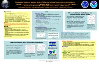
Microwave Applications using CRTM. Benjamin T. Johnson ( UCAR @ NOAA ) Contributions from many CRTM applications / developers. CRTM Workshop , College Park, May 2017. Overview. Microwave Radiative Transfer Theory Emission / Absorption Transmission Scattering CRTM approach Technique

E N D
Microwave Applications using CRTM Benjamin T. Johnson (UCAR @ NOAA) Contributions from many CRTM applications / developers CRTM Workshop, College Park, May 2017
Overview • Microwave Radiative Transfer Theory • Emission / Absorption • Transmission • Scattering • CRTM approach • Technique • Limitations • Examples from CRTM • Imager, Sounder, Radar • Impact of PMW DA on Forecast
Electromagnetic Wave Electromagnetic Radiation :: Wave Electromagnetic Radiation in wave form Source: http://spot.pcc.edu/
Electromagnetic spectrum 1 mm 1 m Range: 1 mm to 1 m (300 GHz to 0.3 GHz) Far Infrared transitions to microwave at about 1 mm (300 GHz). Microwave-centric researchers refer to wavelengths less than 1 mm as “sub-millimeter” (down to about 0.3 mm at 1000 GHz). On the other end, radio waves start around 1 meter wavelength, but there’s no real “transition”, like IR to microwave, it’s a continuous change.
Infrared Microwave radiance spectrum Microwave
Radiative Transfer Overview • How does radiation interact with the atmosphere and surface? • Transmission • Extinction • Scattering + Absorption = Extinction • Extinction Law • Reflection from the Surface • Albedo • Absorption/Emission from the Surface • Radiative Transfer Equation
Radiative Transfer (in words) Radiative Transfer is the process by which electromagnetic radiation propagates from a “source” to a “sink”. Source mechanisms (add radiance along a path): • thermal emission: creation of radiation • transmission: propagation of existing radiation • scattering: outside radiation scattered into path Sink mechanisms (subtract path radiance): • absorption: radiance is absorbed by material • scattering: radiance scattered out of path
Radiative Transfer :: Transmission • Transmission • The portion of radiation incident on a medium / interface that passes through the medium without changing direction (t = transmittance) I0 Ds Inew = t(Ds) I0
Radiative Transfer :: Extinction • Extinction = Scattering + Absorption • The portion of radiation incident on a medium that is not transmitted, but is scattered or absorbed r I0 I0 Ds Inew = t(Ds) (1-r) I0
Radiative Transfer :: Scattering Rayleigh Scattering • Scattering • x = size param. • r = radius • l = wavelength Mie Scattering Mie Scattering -> Geometric Optics
Radiative Transfer :: Surface reflections Specular Reflection Diffuse Reflection (never occurs anywhere in reality, but it’s a convenient approximation)
Forward Model • A forward model is a simulation of the solution of the forward problem, which is simply “solving” the RTE. • Typically, the forward model seeks to simulate what the satellite would observe given a simulated state of the scene of interest. • Example: a cloud-resolving model simulates the physical state of the surface and atmosphere. • These physical properties are associated with radiative properties (scattering, absorption, reflection, emission, etc.) • These properties are placed into a radiative transfer model (a simulation of the RTE), and solved for the radiance within a given field of view (i.e., what a remote sensor would observe). • Result: Simulated satellite observations & “known” geophysical quantities that contribute to the observations
Thermal Radiative Transfer (nonscattering) [1/3] • From Lambert’s law, the change of radiance, I, along a path ds due to absorption is proportional to the amount of matter in the path: • Similarly for emission • βa = volume absorption coefficient • J = source function. • Total change in radiance due to interaction of radiation and matter is then, • This is Schwarzchild’s equation ka = mass absorption coefficient ρ = density Is the Planck function, B(T), under LTE in a non-scattering medium With apologies to Max Planck, ka encompasses all the interesting physics Petty, G.W., 2004, “A First Course in Atmospheric Radiation”, Sundog Publishing, Madison WI. Goody, R.M. and Y.L. Yung, 1989, “Atmospheric Radiation: Theoretical Basis”, 2nd Ed, Oxford University Press, New York.
Thermal Radiative Transfer (nonscattering) [2/3] • This is where we define the optical thickness between two points along the path: • Using this in Schwarzchild’s equation and integrating the optical thickness thickness from 0 (stoa) to it’s value at the surface (ssfc) : • Manipulation of this expression leads to non-scattering radiative transfer equation (RTE), • where Weighting function Petty, G.W., 2004, “A First Course in Atmospheric Radiation”, Sundog Publishing, Madison WI.
Thermal Radiative Transfer (nonscattering) [3/3] • The gaseous absorption algorithm is the core of the CRTM (or any model). • Regular regression model is used where frequency dependent regression coefficients, ci,v, are used with atmospheric state predictors, Xi, to compute the channel absorption coefficients, • Two algorithms for gaseous absorption • ODAS (Optical Depth in Absorber Space). • A “compact” version of the OPTRAN model. • H2O, O3 absorption only. • ODPS (Optical Depth in Pressure Space). • Optical depths computed on a fixed pressure grid. • Better fitting statistics. • More trace gases: CO2, CH4, N2O. • Enables incorporation of Zeeman model (requires fixed pressure grid). Petty, G.W., 2004, “A First Course in Atmospheric Radiation”, Sundog Publishing, Madison WI.
Thermal Radiative Transfer (w/ scattering) [4/3] RTE with scattering • With scattering the change in intensity, dI, becomes: • where • and • The dIscat term takes into account radiation from any direction being scattered into the sensor field-of-view (FOV), • The CRTM uses a look-up table to obtain scattering optical properties (e.g. extinction coefficient, single scatter albedo, etc) and reconstruct phase functions for the necessary number of streams (angles over which the zenith integration is done) Scattering phase function Petty, G.W., 2004, “A First Course in Atmospheric Radiation”, Sundog Publishing, Madison WI.
Infrared Microwave radiance spectrum Microwave
NOAA Prioritized New Satellites and Sensors • New Sensors Data Assimilation: • (new QC, error optimization, impact assessment on NOAA forecast systems) • JPSS1/2– ATMS and CrIS • GOES-16 – ABI (AMV winds and radiances) • COSMIC- 2 GPS-RO (TBD) • HIMAWARI-8/9 AHI (Dry run for GOES-16 ABI) • GPM /GMI • Megha-Tropiques SAPHIR (WV Sounder) • ISS-RAPIDSCAT (Scatterometer) • GCOMW AMSR2 • SMAP • JASON 3 • Existing Sensors optimization: • (QC, Surface-sensitive channels assimilation, pre-processing, dynamic emissivity, etc) • ATMS, SSMI/S, AMSU, MHS
Forward Model Examples [6 hr window] Analysis TBs SSMI/S F18 183.31 +/- 6.6 GHz
Forward Model Examples [5 days] Analysis TBs AMSUA N19 89.0 V GHz
GMI 1C-R VO3A TBs // orbit: 420 // 26-Mar-2014 15:56:38 UTC [K] 10.65V 10.65H 18.7V 18.7H 23.8V 36.5V 36.5H 89.0V 89.0H 166V 166H 183±3 183±7 MRMS
Community Surface Emissivity Model (CSEM) • An open-system with optional models for research and operational applications • Subversion controlled modules • OOP Design • It may be used as an independent model system or as a subsystem of upper-level systems, e.g. CRTM. • Evolved from CRTM but with improved model physics and new algorithms • A platform where research • algorithms(models) may be easily implemented, optimized, and coupled with CRTM and tested in GSI • Forward, tangent-linear, and adjoint operators (slide from M. Chen & F. Weng)
NOAA Retrieval Systems using CRTM NOAA Retrieval Systems (using CRTM) • NOAA Unique CrIS/ATMS Processing System (NUCAPS) • regression algorithm for first guess, cloud-clearing radiance (FOR based), coarse vertical distribution(24 levels for T and 21 levels for h2o), step-wise minimization, more for T, h2o, trace gases • Principal Component-based Retrieval (PCR) • compress radiance into pc scores, EOFs represents vertical variation, simultaneous optimal estimation for each FOV, T, h2o, trace gases, and cloud variables. • Snowfall product from H. Meng using ATMS/AMSU/MHS • Microwave Integrated Retrieval System (MiRS/MIIDAPS) • 1D-var approach, using 20 EOFs in total, no ancillary data required, T, h2o, cloud variables
Typhoon Soudelor 3-Dimensional Structure • MiRS (using CRTM) simultaneous retrieval of temperature profile and hydrometeors allows depiction of storm structure S. Korea RR (mm/h) Rain Water w/Retrieved T profile Typhoon Soudelor 6 August 2015 0445 UTC MiRS SNPP/ATMS Japan Core Region Isosurfaces: GW=0.05 mm, RW=0.01 mm Graupel Water w/Retrieved T profile Cross-Section of RW and GW along 21N latitude Slide from: C. Grassotti
ATMS Ice Extent Comparison over the Northern Hemisphere of sea-ice extent and snow cover extent on 21 February 2013 from (left) MiRS-ATMS and (right) the National Ice Center IMS operational analysis. Boukabara et al., 2013; JGR
Community Hydrometeor Model (CHYM) GFS or User Particle Size Distribution (PSD) In CRTM at CRTM_CloudCoeff.f90 Processed by CRTM as standard CloudCoeff
Community Hydrometeor Model (CHYM) Single-particle database example: The physical database contains 2126 pristine particle files, based on the above 9 base shapes, ranging from columns to plates to dendrites. Effective radius ranges from 60 to 1000 microns. The aggregate particle database, based on aggregates of the 9 base shapes above, consists of about 8100 aggregate shapes, with varying masses and constituent ice crystals. Effective radius ranges from 100 microns up to 5000 microns.
Single-Particle Scattering Tables K.-S. Kuo, NASA GSFC Aggregate particle scattering / extinction properties Pristine particle scattering / extinction properties For each of these files, the current database has scattering and extinction properties are calculated at 13 microwave frequencies: 3, 5, 11, 14, 19, 24, 36, 89, 94, 150, 166, 176, 180, 186, and 190 GHz. Interpolation between frequencies is possible, although a linear assumption is implied. Extrapolation is not advisable outside of the 3-190 GHz range
Texas A&M (P. Yang group) MC-6 particles Hex Plate Agg. (5) Droxtal Oblate Spheroid Hex Plate Hex Column Agg.(8) Solid Hex Column Bullet Rosette Prolate Spheroid Solid Hex Column Hollow Hex Bullet Rosette Hex Plate Agg. (10) Hollow Hex Column Sphere
TAMU MC6 2016 Extinction Efficiency (Qext), all shapes, all frequencies (colorbars) Qext vs. Equivalent Radius (Re) Qext vs. Size Parameter 1mm 1cm scattering dominant regime
Forward Modeling :: Radiances • Simulated passive microwave radiances from 3-D cloud resolving model data (89 – 183.31 GHz)
Influence of Shape on TBs @ 89V - - - Passive Microwave Retrieval of Ice-Phase Precipitation 33/40
CRTM Radar Modeling Status (1/2) • CASM: Community Active Sensor Module (ongoing) • Overarching Goal: Provide a community module for active sensor forward operators. • Current Goal: Provide the ability to simulate radar reflectivity and 2-way path-integrated attenuation (PIA) at any pressure-grid box using CRTM. • CASM Applications: • Forward modeling of active radar reflectivities under all-sky conditions • Direct data assimilation of radar reflectivities in clouds / precipitation • Applicable to satellite-based nadir-viewing radar under the current formulation, but could be applied in low attenuation conditions to an arbitrary radar
CRTM Radar Modeling Status (2/2) • Current limitations: • Reflectivities and PIA limited to vertical until we implement slant-path or arbitrary-path RT • no specific polarization information yet • assumes pressure grid boxes uniformly filled with cloud / precipitation (e.g., no assumptions about non-uniform beam-filling/NUBF) – possible cloud fraction approaches later, but need 3D cloud fraction. • Code status: • Cloud Coefficient generation codes have been modified to produce CloudCoeff.bin files that contain a mass backscattering coefficient (implementation is similar to the mass extinction coefficient) (100%) • Plumbing for CRTM to read new CloudCoeff filetypes, pass the backscattering coefficient through CRTM, reflectivity structure ready (TL/AD) (90%) • The reflectivity equation itself not yet coded, but each element is available:
CRTM Radar Modeling expectations CRTM Simulation (a) CASM (Sim.) Zm[dBZ] @ Ku-band (14 GHz) (b) GPM DPR (Obs.) Zm[dBZ] @ Ku-band (14 GHz) Observed Reflectivities
Fractional Impact at 00UTC: Satellite Radiances = microwave sensors
NASA/GMAO: GEOS FP Observation Impact All Data Types 1 May 2015 – 30 April 2016 00UTC 24h Global Moist Energy Norm microwave sensors Fractional Total Impact Observation Count ~4.3 million totalobservations at 00z
NASA/GMAO: GEOS FP Radiance Impact GEOS FP Observation Impact Monitoring Satellite Radiances 1 May 2015 – 30 April 2016 00UTC 24h Global Moist Energy Norm Fractional Total Impact Observation Count No longer assimilated ~3.0 million radiance observations at 00z