Advanced Assessment Methodology for Thermodynamic Data Optimization
390 likes | 418 Vues
Learn how to systematically optimize thermodynamic data through literature searching and parameter calibration for accurate modeling. Utilize critical assessment and error exclusion techniques for reliable results.

Advanced Assessment Methodology for Thermodynamic Data Optimization
E N D
Presentation Transcript
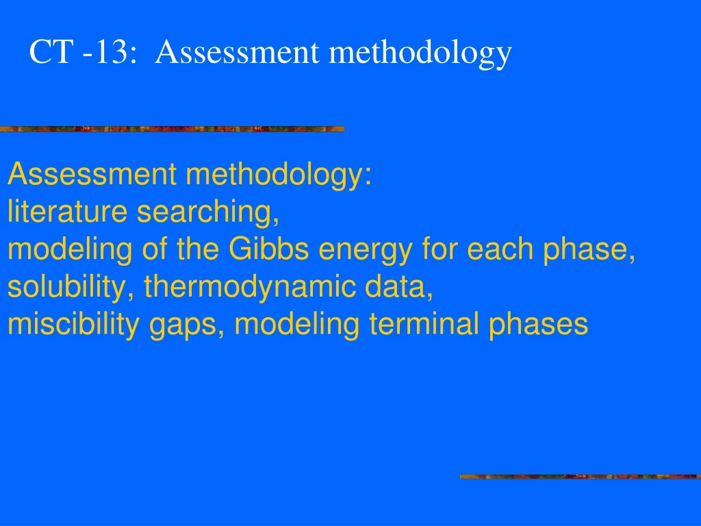
CT -13: Assessment methodology Assessment methodology: literature searching, modeling of the Gibbs energy for each phase, solubility, thermodynamic data, miscibility gaps, modeling terminal phases
Starting the assessment Theaim: Searchforthe model bestable to describeexperimental evidence (thermodynamic, phaseequibrium data, ab initiocalculations) by proper parameters Creatingofanalyticaldescription (findparameters) representingbest set ofparametersdescribingallexperimental data (thermodynamicandphaseequilibrium data) – optimization. Systematicerrorsmustbeexcludedfromoptimizationprocedure (subjectivejudgment are required) – assessment. New experimental evidence requires a newoptimization Assessmentlogbookcontainingallinformation on successandfailuresduringassessmentisveryuseful (thoseinformation are not published in finalpapers) Base forassessment = criticalassessmentofavailableliterature Example: search in JournalofPhaseEquilibriaandDiffusionorothersources
Thermodynamic data (H,G,S) ( H 1 kJ.mol-1, G 1 kJ.mol-1) Parameters in CEF (G,L) ??? Phase diagram (T,xi) (T 5 K, xi 0.01 mol.%)
Literature searching Relevant journals: CALPHAD, Zeitschrift für Metallkunde (now International Journal of Materials Rersearch), Journal of Alloys and Compounds, Intermetallics, Thermochimica Acta, Physical Review B, Philosophical Magazine, Acta Materialia, Metallurgical and Materials Transactions, Nature Materials, Acta Crystallographica and Scripta Materialia. Also the literature quoted in JANAF tables or in critical evaluation of the International Programme for Alloy Phase Diagram Data may be useful in this stage. Electronic access via Web of Science, Chemical Abstracts or Scopus enhances to find relevant papers on given topics. It is a rule to obtain all original papers first!
Literature searching – cont. • It is a rule to obtain all original papers first! • Originally measured quantity is often reported after having been transformed! It may contain more information than is in reported tables and curves. • Clasification of data by types: • Experimental thermodynamic data (calorimetry, emf, vapor-pressure methods) • Experimental phase diagram data (thermal analysis, metallography, X-ray • diffraction, SEM-EDX, diffusion couple experiments) • Other experimental data (bulk moduli, thermal expansion, elastic constants…) • Crystal structure data, point defects, density, ordering, resistivity, vibrations… • Theoretical calculations of total energies at 0 K, estimates, trends, • thermodynamic properties and phase diagrams of similar systems…. • Review papers, critical assessments, and previous optimizations • Miscellaneous • Example: MATPORT – Landolt-Börnstein New Series (Fe-Mn-Cr, Fe-Mo-W) • Reviewer‘s Guide
Analysis of experimental data Detection of contradictory data in literature (different value for the same quantity) Dataset with systematic errors must be excluded. No general rule exist! Description of experimental procedure may help (reaction with crucible material, evaporation of volatile component or not reaching equilibrium) Arguments for categorizing set of data must be clearly specified in publication! Errors in the literature data may reveal after first trials of optimization – categorizing of data must be repeated! For values unique to a system: it is recommended to select „best“ value for optimization (least-square method find a mean of all values. „Best“ value can be changed in the course of optimization.) Data should not be smoothed before optimization treatment. It importes subjective preference to the process. Ternary phase-diagram data (temperatures at which solid phase appears at cooling) should be interpreted with great care (composition of liquid phase will change while the solid phase is precipitating – see Scheil simulation).
Requirements for using the Least Square Method • The randomness of the observed quantities has a Gaussian probability distribution • The observed quantities are only subject to random errors • The different experiments are uncorrelated • The standard deviation of each observation can be estimated • The number of observation is large • The considered models are exact Usually not fulfilled in any thermodynamic assessment but we can try to approach as close as possible.
Phase equilibrium dataSelection of the set of phases to be considered Liquid phase – allways present Terminal phases – pure elements with varying homogeneity ranges Intermediate phases – intermetallics, oxides, carbides etc., - phases may be metastable (e.g. cementite in Fe-C system, they must be included in the optimization) - identification of phases: X – ray single-crystal diffraction (neutron diffraction for the case of similar scattering of X-rays by different atoms of alloy) Problem with two-phase sample Problem with not reaching equilibrium (missing phase after not long enough annealing, detecting metastable phase after quenching) Result of this step is a table, indicating which kind of experimental data are known for each phase - example
Selection of the set of phases to be considered - example LFS - CT
Modeling the Gibbs energy for each phase Each phase can be modeled independently, but phases with the same crystal structure can be modeled as the same phase General considerations Gibbs energy should be described by a model presented during this course. Models presented here have physical background and experimental data must fit the corresponding calculated quantity well using only a few model parameters. Some of the polynomial excess terms are only curve-fitting formulae to be used for description of small deviations from the model. No model is able to take into account all possible physical effects. (All models contain simplifications.) For the selection of the model, enthalpies and chemical potentials (activities) in single phase region are most important. The more complicated a description, the more unpredictable the extrapolation. Modeling the phase may have to be compatible with existing multicomponent databases. Each phase is characterized by prototype crystal structure and it is important to find phases with the same prototype in other systems (namely in intermetallic phases) e.g. for possible mutual solubility.
Solubility and composition range Liquid is often stable across the whole composition range and even if there is miscibility gap, the same model should be used on both sides of the miscibility gap. Terminal phase may also be stable across the whole composition range if the pure elements have the same crystal-structure type. Terminal phases, having the same structure, must be modeled as the same phase even if there is miscibility gap and stable intermediate phase are in between terminal phases. All phases have some range of solubility. Phase with small range of solubility may be approximated by stoichiometric compound, which is much more simpler to model (e.g. graphite). Importance of solubility limit is different: in semiconductor phase, it is important to model solubility of 10-6 mole fraction, in metallurgy, 10-3 mole fraction is important. For intermetallic phases – sublattice model describes small solubility ranges (e.g. Laves phases) Phases with wide solubility ranges may have ordering inside their composition ranges (e.g.A2/B2 ordering). It is possible to prove it by activity a(xi) measurements.
Solubility and composition range-example Relations betweenGibbsenergycurvesandphase diagram are shown. b LFS - CT
Phase diagram Cu-Zn: A.Dinsdale, A.Watson, A.Kroupa, J. Vrestal, A.Zemanova, J.Vizdal: Atlas pf Phase Diagrams for Lead-Free Soldering. COST 2008, Printed in Brno, Czech Rep. Solubility and composition range-example Second-ordertransition BCC_A2B2_BCC isconcentrationdependentandliesbetween 454-467 oC LFS - CT
Thermodynamic data General considerations: Enthalpy of mixing H(x) curve has „V“ shape – strong LRO or SRO should be expected, defects and associates contribute to the (excess) heat capacity Enthalpy of mixing (formation) H(T) has no significant temperature dependence – Kopp-Neumann rule is valid (no excess heat capacity should be modeled) Partial enthalpies and chemical potentials: drastic change in small composition range indicates ordering. Description of B2/A2 or L12/A1 ordering is possible Modeling of integral molar enthalpies by Redlich-Kister (RK) polynomial with zero excess entropy is proper for phases without tendency to LRO, temperature dependence of integral and partial molar enthalpies and Gibbs energies can be neglected (Hm = Gm is allways valid at 0 K): Hm = Gm = n-1inj=i+1 xixj(k=0(xi – xj). Lij ) Drastic temperature dependence of second derivative of Gibbs energy („phase stability“) cannot be modeled by Redlich-Kister polynomial (for mathematic reasons!), but Wagner-Schottky model (or associate-solution model or ionic-liquid model) should be used („V“ shape curves)
Thermodynamic data - example L used: L0 L0, L1 L0, L2, L4 LFS - CT Modeling ofintegralmolarenthalpies by Redlich-Kisterpolynomialwithzeroexcessentropy (Hm = Gm) column 1-3. Wagner-Schottky model for LRO isdemonstrated (column 4). SecondderivativeofGibbsenergy („phase stability“) isshown in lowest line.
Estimation methods Kopp-Neumann rule for heat capacities of compounds (Kopp 1864, Neumann 1865): Cp,AaBb a.Cp,A + b.Cp,B (It may be used for solutions also.) Tanaka‘s rule for entropy of liquid solutions (T. Tanaka, N.A. Gokcen, Z. Morita, Z. Metallkde 81 (1990) 49): HM/SE Tm (Tm is melting temperature of phase) Miedema‘s guess of enthalpy of formationof liquid phase and compounds F.R. De Boer, R. Boom, A.R. Miedema, Physica 113B (1982) 18-41 First-principle total-energy calculations, using DFT (density functional theory) methods at 0K, provide values of enthalpy of formation of real compounds (ordered compounds) as well as fictitious end members in CEF. Systematic behavior – comparison with similar but well known systems can be a good guide.
Modeling of the gas phase and the liquid phase • Gasphase: differentassessmenttechniques – thermodynamicdescriptionsofgaseousmoleculescanbeobtained by ab initiocalculationsorfromspectroscopic data (Database SGTE, Landolt-Börnsteinseries) • Liquidphase: descriptipon in wholecompositionrange, type ofbondingmaychangewithtemperatureandcomposition: mixHliq(x)shouldbeconsidered in the modeling! Formainlymetallicor van der Waalsbonding (direction-independent) – regularsolutionisgood model and RK polynomialisused as curve-fittingformula. • Deepeutecticsbetweentwointermediatephases (e.g. Mg-Znsystem) mayexist. • Shapeofliquiduscurvemaydiffersignificantly on thetwosidesof a congruentlymeltedcompound. Itcanbeexplained on the base ofGibbs-Konovalov rule: • (dT/dx)coex= [(x - x) T (2Gm / x2)] / [(H1- H1) (1- x) + (H2- H2) x]
Miscibility gaps Liquid metal-oxygen system have often wide miscibility gap. Example: Cu-S system has a miscibility gap between Cu-rich liquid and liquid with average compostion Cu2S (associate), which survive in Cu-Fe-S system. Single model must be used. Example: Cu-Fe, Cu-Co systems has liquidus almost horizontal for a significant composition range. That is an indication of a metastable miscibility gap just below the liquidus.
Miscibility gaps-example Two liquids T/oC XS Cu – S system M.Hansen, K.Anderko: ConstitutionofBinaryAlloys. McGraw-HillBook Co., New York, 1958
Miscibility gaps-example FCC(Cu) + FCC(Fe) FCC metastablemiscibility gap I.Ansara, A.Jansson: Trita-Mac-0533, 1993, KTH, Stockholm
Miscibility gaps-example FCC(Co) + FCC(Cu) FCC metastable miscibility gap J.Kubišta, J.Vřešťál: Journal of Phase Equilibria 21 (2000) 125-129
Short-range ordering (SRO) in liquids A „V“ shaped enthalpy of mixing vrt. mole fraction curve = evidence of SRO, its apex indicates the stoichiometry of an „entity“ (atomic configuration that appears statistically more frequently than others). In the phase diagram this apex often matches by congruently melted phase at the same composition. Example: Mg-Sn and Pb-Te systems If „V“ shaped enthalpy of mixing vrt. mole fraction curve is less pronounced – several different cations or anions may exist and RK series may still be sufficient as curve-fitting formula. If bonding is less pronouncedly covalent or ionic, the „V“ shaped enthalpy may be an indication of SRO and quasi-chemical approximation may be used with non-random entropy of mixing. It is equivalent to excess entropy term in RK formalism, which is a curve-fitting method only. It does not describe the excess heat capacity connected with the decrease in enthalpy of formation due to the decrease of SRO on heating.
Short-range ordering (SRO) in liquids - example T / oC Sn wt.% 1300 K 700 K xSn and its phase diagram LFS - CT
Short-range ordering (SRO) in liquids - example T / oC xTe and its phase diagram LFS - CT
Freezing point depression (cryoscopy) The depression of the melting temperature Tf of pure A on adding B,(when there is no solubility of B in A), is: xBL = (HfA/(RT)) ((Tf – T)/Tf) (van‘t Hoff law) It is independent on alloying element (it is dependent on solvent only). If experimental information for liquidus reveals a strong deviation from the slope given by this equation, it is indication, that one mole of added element corresponds to a different number of moles of dissolved species.
Modeling terminal phases Terminal phase = phase which exists with a pure component of the system. Solubility ranges may vary. It is useful to describe the Gibbs energy such phase for the whole composition range. If the element has different crystal structures, then Gibbs energy of a metastable state (lattice stability) of the element must be related to that of it stable state (SER). These relationships form a unary database. First version of it: A.T.Dinsdale, CALPHAD 15 (1991) 317-425, it is regularly updated. Agencies producing databases provide it in electronic form free of charge.
Modeling substitutional solutions Terminal phases: important for modeling without intermediate phases, • often the RK formalism is appropriate: complete solubility • across the whole concentration range may exist (e.g. Cr-V, • Ag-Au, Ag-Pd). • Difference in atomic sizes (e.g. Ag-Cu) and chemical • properties create miscibility gap or intermediate phases • which interrupt the solubility range (e.g. Cr-Mo, Fe-Mo). • Check the modeling of terminal phases during assessment, by calculating the metastable phase diagram with just terminal phases, is possible. • Some components may form ordered phases based on the same lattice as the terminal solution.
Modeling substitutional solutions-example Phase diagram of the Fe-Mo system
Modeling interstitial solutions BCC lattice: (carbon in ferrite) – octahedral interstitial sites at the middle of the edges and at the centers of planes of the unit cell – three times as many interstitial sites than matrix atom sites Sublattice model is: (Fe, Cr, …)1 (Va, C, N)3 FCC lattice: (carbon in austenite) – tetrahedral interstitial lattice sites and octahedral ones. Carbon and nitrogen dissolve in the octahedral sites only. Sublattice model: (Fe, Cr, …)1 (Va, C, N)1 HCP lattice: (oxygen in titanium) – one octahedral site per matrix atom, but old modeling (deduced from carbides like W2C) with only half intersticial sites is stil used Sublattice model is: (Fe, Cr, …)1 (Va, C, N, O)0.5 Parameters in CEF: GMe:Va – unary data, GMe:X – fictitious value, LMe:Va:X – adjust composition dependence of the Gibbs-energy description. For GMe:X, an arbitrary and large enough positive value or linear function of T is chosen and oLMe:Va,X is used to adjust the Gibbs energy in the range of homogeneity.
Modeling of ordering phenomena Ordering of crystal structure by adding elements: Fe-Al system: Adding Al to Fe change occupation of Al in an Fe bcc lattice from disordered A2 to ordered B2. It is second-order transition (it appears gradually and no two-phase region between A2 and B2 phase exists.) Similar process is ferromagnetic transition – (see example) Al-Ni system: Other type of ordering, where the occupancy of the fcc lattice changes the structure from the disordered A1 to ordered L12 type (Ni3Al). The ordered phase appears as a separate intermediate phase in the phase diagram (first-order transition). Both phases can be described by the same Gibbs-energy function (partitioning).
Modeling of ordering phenomena - example M.Hansen, K.Anderko: ConstitutionofBinaryAlloys. McGraw-HillBook Co., New York, 1958 Orderingtransitionof Ni3Al not denoted.
Metastable interpretation of terminal phases Proposed and done by J.J.van Laar (1908), currently standard procedure in the assessments, namely for multicomponent databases: When terminal phases do not extend across the whole system (due to miscibility gap or due to intermediate phases) it is interesting to extrapolate the metastable two-phase field between the liquid and terminal phases using the assessed parameters. Strange curvatures reveal mistakes in coefficients in the RK series for one or both phases (e.g. to many coefficients).
Metastable interpretation of terminal phases - example LFS - CT
Terminal phases in quasibinary systems Quasibinary system is a system with three components that behaves exactly like a binary system of two components (components are bound in compounds). Example: MgO – CaO system: NO = NMg +NCa – two independent components. Quasibinary system must have the endpoints of the tie-lines betwen the phases inside the section defined by quasibinary components (in the plane of the section!). Example: CaO-FeO: Fe is always mixture of Fe2+ and Fe3+, diagram is called „pseudobinary“ instead of „quasibinary“ – endpoints of tie-lines will be slightly outside the composition plane defined by compounds Problem with activity of oxides may arise when different quasibinary components are defined (Al2O3 instead of AlO1.5) because the activity of the species is the product of the activities of atoms contained in the species (chemical potential of Y2O3 is twice that of YO1.5).
Example: Assessment of the Bi-Pd System Phase diagram and structure data: J.Brasier, W.Hume-Rothery: J.Less-Common Metals 1, 157 (1959) Pauling file – Pearson‘s Handbook – P.Villars P.Oberndorff: PhD Theses, TU Eindhoven 2001 No thermodynamic information available – therefore enthalpy of mixing of liquid Bi-Pd alloys was measured: published in: J.Vrestal et al.: Calphad 30(2006)14-17
Example: Re-optimization of Ag-Pd system • New data for enthalpy of liquid phase published • (2005) • New data for solid-liquid equilibrium and • new data for activity of Ag in liquid phase added – paper is accepted in J. of Alloys and Comp.
Questions for learning 1. Explain the terms „optimisation“ and „assessment“ 2. Describe the process of assessment 3.Describe the process of selecting of experimental data and their testing 4.Describe the process of modeling of terminal phases, intermediate phases, substitutional solutions and interstitial solutions 5. Describe the process of modeling of ordering phenomena