Overview of Turbulent Flux Parameterizations for Air-Sea Interaction Modeling
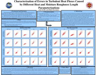
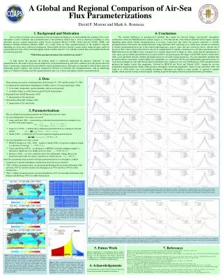
This article provides a comprehensive breakdown of six turbulent flux parameterizations used in air-sea interaction modeling, categorized into sea-state independent and sea-state dependent types. It discusses the parameterizations by Large and Pond, Smith, HEXOS, Taylor and Yelland, and Bourassa, highlighting their differences in accounting for wind speed regimes and roughness length. Furthermore, it examines how these flux parameterizations interact with atmospheric stability assumptions, featuring various stability parameterizations. This understanding aids modelers in selecting appropriate flux parameterizations for specific oceanic contexts.

Overview of Turbulent Flux Parameterizations for Air-Sea Interaction Modeling
E N D
Presentation Transcript
3. Parameterizations The six turbulent flux parameterizations are broken down into two types: • sea-state independent (wave data is not used) • Large and Pond (1981) - a neutral drag coefficient parameterization accounting for two possible wind speed regimes: • Large et al. (1994) – a neutral drag coefficient parameterization accounting for all wind speeds: • Smith (1988) – a Charnock (1955) based roughness length parameterization: • sea-state dependent (wave data is used) • HEXOS (Smith et al. 1992, 1996) – similar to Smith (1988), except that roughness length is a function of waveage: • Taylor and Yelland (2001) – an alternative to HEXOS, such that roughness length is a function of significant wave height and wave slope: • Bourassa (2006) – sea state contributes the lower wind profile, adding shear to the horizontal wind at the sea-surface, expressed as orbital velocity: Each flux parameterization is mated with three parameterizations for atmospheric stability: • Assumption of neutral atmospheric stratification above the air-sea interface. • “Old” stability parameterizations, incorporating the Businger-Dyer relations (Businger 1966 and Dyer 1967 for unstable stratification; Businger et al. 1971 and Dyer 1974 for stable stratification). • “New” stability parameterizations, incorporating Benoit (1977) for unstable stratification and Beljaars and Holtslag (1991) for stable stratification. Figure 4: Global probability distribution functions are displayed separately for all six turbulent flux parameterizations and for all five flux diagnostic variables: latent heat flux, sensible heat flux, stress, friction velocity cubed, and the curl of the stress. Each PDF is individually broken down by a Bulk Richardson range for atmospheric stability, delineated by color. Fluxes derived from each of the three stability parameterizations are delineated by line type (solid, dashed, and dashed-dotted). PDF diagrams that appear to have only the solid line type (i.e. the neutral assumption), are due to an exact overlap from other stability parameterizations, suggesting that stability parameterizations produce virtually no difference for that given flux. 70.5% Figure 5: Regional probability distribution functions for the Gulf Stream are displayed separately for each turbulent flux diagnostic: latent heat flux, sensible heat flux, stress, friction velocity cubed, and the curl of the stress. Turbulent flux output is represented by all six turbulent flux parameterizations, representing only the output from the “New” atmospheric stability parameterizations. The upper diagrams depict the summer season, and the lower plots depict the winter season. For brevity, intermediate seasons and the output from remaining atmospheric stability parameterizations are left out. 4.1% 22.3% 3.1% 3.1% Figure 1: The standard deviations from the composite mean interquartile range of latent heat flux, sensible heat flux, and stress are shown respectively. Boxed regions highlight areas of interest, where probability distribution functions will be used to determine modeled flux output differences. The Kuroshio, Gulf Stream, SW Indian Ocean, and SW Pacific Ocean are chosen based upon their high modeled latent and sensible heat flux variability. Drake’s Passage is chosen to better understand the response of heat fluxes to the highly variable stress in the ACC region. The Equatorial Cold Tongue is a predetermined area of interest, which appears to show the least modeled flux variability among the remaining regions. Figure 3: Shows a probability distribution function of the Bulk Richardson numbers, derived from the CORE and Reynold’s SST datasets. Colors delineate the Bulk Richardson stability ranges. Percentages marked within the diagram show the relative contribution of the total distribution of stability ranges. Since the y-axis is logarithmic, the scale of each stability range is exaggerated. 1. Background and Motivation Air-sea fluxes of energy and momentum are the most important diagnostic for understanding the coupling of the ocean-atmosphere system. Turbulent flux parameterization is the preferred method that is used in numerical modeling to more efficiently process coupled interactions within Ocean Circulation Models (OCM), Global Spectral Models (GSM), and Numerical Weather Prediction Models (NWP). As a result, there are many parameterizations at the modeler’s disposal, depending on a wide array of physical assumptions. Each modeler also has a specific oceanic region, temporal range, and/or an assumed physical state of the ocean/atmosphere suited to his/her interests. It is with this in mind, that each modeler should ask the following question: “Which flux parameterization is best suited for my needs?” To help answer this question, the modeler needs to collectively understand the physical “make-up” of each parameterization, the relative biases that are induced by each parameterization, and what conditions pose the greatest threat in terms of generating a high model bias provided by a given parameterization. This project is intended to address these issues by performing global, regional, and seasonal comparisons between six turbulent flux parameterizations, with an underlying analysis of stability by mating each flux parameterization with a set of three atmospheric stability parameterizations. 4. Conclusions The smallest differences in parameterized turbulent flux output are observed during “near-neutral” atmospheric stratification, where the Bulk Richardson stability range is +/- 0.02. Beyond this “near-neutral” threshold, fluxes begin to diverge depending upon which stability parameterization is in place. Latent heat flux shows the greatest sensitivity to stability parameterizations, followed by the sensible heat flux. Large and Pond (1981) and Large et al. (1994) show virtually no sensitivity to stability parameterizations in any of the wind forcing diagnostics, such as: stress, the cube of friction velocity, and the curl of the stress; this is due to the fact that friction velocity is computed prior to stability calculations for only these parameterizations. RMS differences for the IQR of stress, averaged over a specific region (refer to Figure 2), show clearly that the dependencies of stress upon a given stability parameterization are quite small for any given region; this aligns with the PDF analysis which shows really good agreement between stability parameterizations for all wind forcing diagnostics. Sea-state dependent turbulent flux parameterizations consistently compute higher flux magnitudes (as compared to the sea-state independent parameterizations) for each observed diagnostic; the Gulf Stream analysis illuminates this comparison very well. The Bourassa (2006) parameterization produces the highest overall flux magnitudes, followed by HEXOS and Taylor and Yelland (2001). Among the sea-state independent parameterizations, Smith (1988) produces the highest overall flux magnitudes, whereas Large and Pond (1981) and Large et al. (1994) follow very close together throughout. Differences are higher in winter months, as opposed to summer months, where episodic forcing is more frequent, resulting in greater divergence between parameterized flux possibilities. A Global and Regional Comparison of Air-Sea Flux ParameterizationsDavid F. Moroni and Mark A. Bourassa • 2. Data Three datasets are used in calculating fluxes from January 30, 1997 until December 31, 2004: • Coordinated Ocean Reference Experiments (CORE) version 1.0 (Large and Yeager, 2004) • 10 m winds, temperature, specific humidity, and sea-level pressure • Available 4x/day on a T62 Gaussian grid (192x94 lon/lat points) • Reynolds Daily OI SST (Reynolds, 2006) • Interpolated to T62 and 4x/day • NOAA Wave Watch III (Tolman, 2002) • Interpolated to T62 and 4x/day LP81 Large94 Smith88 HEXOS TY01 Bourassa06 SW Indian 0 0 0.001035 0.001563 0.00096 0.00152 SW Pacific 0 0 0.001452 0.002064 0.001343 0.002145 Drake's Passage 0 0 0.000599 0.00088 0.00067 0.000891 Cold Tongue 0 0 0.000696 0.000913 0.000541 0.001056 Kuroshio 0 0 0.002846 0.003837 0.002895 0.004176 Gulf Stream 0 0 0.002117 0.003022 0.002191 0.003408 Neutral New Old SW Indian 0.029899 0.030619 0.030692 SW Pacific 0.019858 0.021313 0.021397 Drake's Passage 0.039358 0.039893 0.039962 Cold Tongue 0.010037 0.010541 0.010568 Kuroshio 0.022257 0.025305 0.025499 Gulf Stream 0.025819 0.028347 0.028537 Figure 2: Both charts represent the RMS difference of the IQR for stress, averaged over a specified region. The top chart holds a given drag coefficient parameterization constant, while accounting for all stability parameterizations. The bottom chart holds a given stability parameterization constant, while accounting for all six drag coefficient parameterizations. 5. Future Work Include comparisons for each remaining region of interest: Kuroshio, SW Indian Ocean, SW Pacific Ocean, Drake’s Passage, and the Equatorial Cold Tongue. Include the COARE version 3.0 algorithm and the polynomial curve fit to COARE (Kara et al. 2005) in the PDF analysis. • 7. References • Beljaars, A. C. M., and A. A. M. Holtslag, 1991: Flux parameterization over land surfaces for atmospheric models, J. Appl. Meteor.,30, 327-341. • Benoit, R., 1977: On the integral of the surface layer profile-gradient functions. J. Appl. Meteor., 16, 859-560. • Bourassa, M. A. 2006, Satellite-based observations of surface turbulent stress during severe weather, Atmosphere - Ocean Interactions, Vol. 2., ed., W. Perrie, Wessex Institute of Technology Press, 35 – 52 pp. • Businger, J. A., 1966: Transfer of momentum and heat in the planetary boundary layer. Proc. Symp. Arctic Heat Budget and Atmospheric Circulation, the RAND Corporations, 305-331. • ______, J. C. Wyngaard, Y. Izumi, and E. F. Bradley, 1971: Flux profile relationships in the atmospheric surface layer. J. Atmos. Sci., 28, 181-189. • Charnock, H., 1955: Wind stress on a water surface. Quart. J. Roy. Meteor. Soc., 81, 639-640. • Dyer, A. J., 1967: The turbulent transport of heat and water vapour in an unstable atmosphere. Quart. J. Roy. Meteor. Soc., 93, 501-508. • Dyer, A. J., 1974: A review of flux-profile relationships. Bound.-Layer Meteor., 7, 363-372. • Large, W. G., and S. Pond, 1981: Open ocean momentum flux measurements in moderate to strong winds. J. Phys. Oceanogr., 11, 324—336. • ______, J. C. McWilliams, S. C. Doney, 1994: Oceanic vertical mixing: a review and a model with a nonlocal boundary layer parameterization. Rev. Geophys.,32. 363-403. • ______, and S. G. Yeager, 2004: Diurnal to decadal global forcing for ocean and sea-ice models: The data sets and flux climatologies. NCAR Technical Note, NCAR/TN-460†STR, 105pp. • Reynolds, R. W., 2006: Personal communication. • Smith, S. D., 1988: Coefficients for sea surface wind stress, heat flux, and wind profiles as a function of wind speed and temperature. J. Geophys. Res.,93, No. C12, 15,467-15,472. • Taylor, P. K., M. J. Yelland, 2001: The Dependence of sea surface roughness on the height and steepness of the waves. J. Phys. Oceanogr., 31, 572-590. • Tolman, H. L., 2002: Validation of WAVEWATCH III version 1.15 for a global domain. Technical Note. Environmental Modeling Center, Ocean Modeling Branch, NOAA. 6. Acknowledgements I would finally like to thank NOAA’s Climate Observation Division for providing the funding for this project.