Landmark Classification in Large-scale Image Collections ICCV 09
240 likes | 449 Vues
Yunpeng Li David J. Crandall Daniel P. Huttenlocher Department of Computer Science, Cornell University Ithaca, NY 14853 USA. Landmark Classification in Large-scale Image Collections ICCV 09. Outline. Introduction Approach Experiments Summary.

Landmark Classification in Large-scale Image Collections ICCV 09
E N D
Presentation Transcript
Yunpeng Li David J. Crandall Daniel P. Huttenlocher Department of Computer Science, Cornell University Ithaca, NY 14853 USA Landmark Classification in Large-scale Image CollectionsICCV 09
Outline • Introduction • Approach • Experiments • Summary Let’s see the DEMO about the paper we discussed last two weeks http://www.zhaoming.name/publications/2009_CVPR_landmark_demo/
Introduction • What is Landmark? • If many people have taken photos at a given location , there is high likelihood that they are photographing some common area of interest , what we call it the Landmark • Recent research in recognition or classification has used Internet resources • But , the test images have been selected and labeled by hand, yielding relatively small validation sets
Introduction Widely-used data sets Goal Consider image classification on much larger datasets (millions of images and hundreds of categories) Develop a collection over 30 million photos , with ground-truth category labels nearly 2 million Ground-truth labeling is done automatically -base on geolocation information
Introduction • Mean shift [3] • Find peaks in the spatial distribution of geo-tagged photos • Use large peaks to define the category labels. • Multiclass SVM [4] • Learn models for various classification tasks on labeled dataset of nearly two millions images • Clustering local interest point descriptors [11] • Use visual features into a visual vocabulary • Using textual tags • Flickr users assign to photos • As additional features [11] D. G. Lowe. Distinctive image features from scale-invariant keypoints. IJCV, 60(2):91–110, 2004. [4] K. Crammer and Y. Singer. On the algorithmic implementation of multiclass kernel-based vector machines. JMLR, 2001. [3] D. Comaniciu and P. Meer. Mean shift: A robust approach toward feature space analysis. PAMI, 2002.
Introduction • Others resource that internet collections also include • Consider the photo stream ,using features from photos taken nearby in time to aid in classification decisions. • use the structured SVM [18] to predict the sequence of category labels • Present a set of large-scale classification involving between 10 and 500 categories and tens to hundreds of thousands of photos • Find that the combinationof image and text features performs better than either alone. [18] I. Tsochantaridis, T. Hofmann, T. Joachims, and Y. Altun. Support vector machine learning for interdependent and structured output spaces. In ICML, 2004.
Related Work • Compare to [8] • We don’t try to predict location but rather just use location to derive category labels. • [8] Test set only contains 237 images that were partially selected by hand • Use automatically-generated test sets contain tens or hundreds of thousands of photos, providing highly reliable estimates of performance accuracy • Very recent work [21] is very similar • However the test set they use is hand-selected and very small – 728 total images for a 124 category problem, or fewer than 6 test images per category • --their approach is based on NN search [8] J. Hays and A. A. Efros. IM2GPS: Estimating geographic information from a single image. In CVPR, 2008. [21] Y.-T. Zheng, M. Zhao, Y. Song, H. Adam, U. Buddemeier, A. Bissacco, F. Brucher, T.-S. Chua, and H. Neven. Tour the world: building a web-scale landmark recognition engine. In CVPR, 2009.
Building Internet-Scale Datasets • Long-term goal • to create large publicly-available labeled datasets that are representative of photos found on photo-sharing sites on the web • Using Flickr API to retrieve metadata for over 60 million geotagged photos • Eliminate photos for which the precision of the geotags is worse than about a city block, remaining 30 million photos. • Perform a mean shift clustering procedure[3] • Downloaded the image data for all 1.9 million within these 500 landmark • Downloaded all images taken within 48 hours of any photo taken in a landmark , bringing the total number of images to about 6.5 million
Approach(visual feature) Adopt the bag-of–features model of [6] , build a visual vocabulary by clustering SIFT descriptors from photos in the training set using the k-means algo. Use Approximate nearest neighbor(ANN)technique [1] to efficiently assign points to cluster centers. Form the frequency vector which counts the number of occurrences of each visual word in the image Normalized L2-norm of 1 The Advantage is it guarantees an upper bound on the approximation error, unlike other techniques such as randomized k-d trees[12] [6] G. Csurka, C. Dance, L. Fan, J. Willamowski, and C. Bray. Visual categorization with bags of keypoints. In ECCVWorkshop on Statistical Learning in Computer Vision, 2004. [1] S. Arya and D. M. Mount. Approximate nearest neighbor queries in fixed dimensions. In ACM-SIAM Symposium on Discrete Algorithms, 1993.
Approach(text feature) At least three different users is a dimension Binary vector indicating presence or absence Normalized L2-norm of 1 Study combinations of image and textual feature Finally, the two feature vectors are concatenated
Approach Let m be the number of classes and x be the feature vector of a photo Note that , the photo is always assumed to belong to one of m categories since this is nature a multiway classification problem
Approach Utilize the multiclass SVM [4] to learn the model w -- using the SVMmulticlasssoftware package [9] A set of training examples Multiclass SVM optimizes the objective function [9] T. Joachims. Making large-scale SVM learning practical. In B. Sch¨olkopf, C. Burges, and A. Smola, editors, Advances in Kernel Methods - Support Vector Learning. 1999.
Temporal info. Outline • Temporal Model for Joint Classification • To learn the patterns created by such constraint • View temporal sequence of photos taken by the same user as a single entity and label them jointly as a structured output • Node Features • Edge Features • Model a temporal sequence of photos as graphical model with a chain topology, where node represent photos and edges connect nodes that are consecutive in time • Overall Feature Map • Parameter Learning
Approach(Node feature) • Feature Map for node v • I(.) is an indicator function • Let be the corresponding model parameter with being the weight vector for class y • Node score
Approach(Edge feature) • Feature vector • Invalid Feature vector • The complete feature map for an edge • Edge score
Approach(Overall Feature Map) • Overall feature map • Total Score • The predicted labeling • This can be obtained efficiently using Viterbi decoding because the graph is acyclic finding the most likely sequence
Approach(Parameter Learning) • The model parameters are learned using structure SVMs [18] • The loss function • The violated constraint
Experiments Involves about 35,000 Test image 12% improvement
Experiments • Human vs. automatic classifier • Asked 20 well-traveled people to each label 50 photos taken at the world’s top 10 landmarks
Experiments • Image classification on a single 2.66 GHz CPU takes about 2.4 sec • Classification requires about 3.06ms for 200 categories 0.15ms for 20 categories • SVM training times , ranging from less than a minute on 10-way problem 72 hour for the 500-way structured SVM on singe CPU • Conducted experiments on a small cluster of 60 nodes Hadoop open source map-reduce framework
Summary • Present a means of creating large labeled image datasets from geotagged image collections • Experimented with a set of over 30 million images of which nearly 2 million are labeled • Multiclass SVM classifiers using SIFT-based bag-of-word features achieve quite good classification rates for large scale problems • Using structure SVM to classify the stream of photos yields dramatic improvement in classification rate • Accuracy that in some case comparable to humans on the same task