Download
1 / 39
460 likes | 2.03k Vues
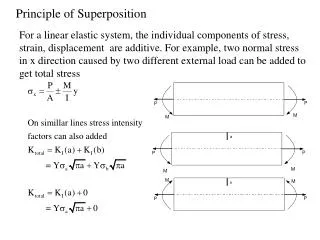
Principle of Superposition. For a linear elastic system, the individual components of stress, strain, displacement are additive. For example, two normal stress in x direction caused by two different external load can be added to get total stress. Principle of Superposition.

E N D
Principle of Superposition For a linear elastic system, the individual components of stress, strain, displacement are additive. For example, two normal stress in x direction caused by two different external load can be added to get total stress
Principle of Superposition For example consider a plate having semicircular crack subjected to an internal pressure
Crack Tip Plasticity LEFM assumes a sharp crack tip, inducing infinite stress at the crack tip. But in real materials, the crack tip radius is finite and hence the crack tip stresses are also finite. In addition, inelastic deformations due to plasticity in metals, crazing in polymers leads to further relaxation of stresses. For metals with yielding, LEFM solutions are not accurate. A small region around the crack tip yields leading to a small plastic zone around it. For moderately yielding metals, LEFM solutions can be used with simple correction. For extensively yielding metals, alternative fracture parameters like CTOD, J-integral are to be used taking into account material non-linearity.
Small Scale Plasticity Irwin’s Approach Normal stress syy based on elastic analysis is given by On the crack plane q = 0 As a first approximation yielding occurs when syy = sys ry = first order estimate of plastic zone size. This is approximate estimate, because of the fact that syy is based on elastic analysis
Irwin’s Approach When yielding occurs, stresses redistribute in order to satisfy equilibrium conditions. The cross hatched regions represents forces active in the elastic analysis that cannot be carried in elasto-plastic analysis, because of the reason that the stresses cannot exceed sys.To redistribute this excessive force, the plastic zone size must increase. This is possible if the material immediately ahead of plastic zone carries more stress. Irwin proposed that plasticity makes the crack behave as if it were larger than actual physical size. Let the effective crack size be aeff , such that aeff = a+d, where d is the correction. or
To permit redistribution of stresses , the areas A and B must be the same
A long rectangular plate has a width of 100 mm, thickness of 5 mm and an axial load of 50 kN. If the plate is made of titanium Ti-6AL-4V,(KIC=115 MPa-m1/2, sys=p10 MPa) what is the factor of safety against crack growth for a crack of length a = 20 mm.
Strip Yield Method (Proposed by Dugdale and Barrenblatt) They assumed a narrow long slender plastic zone ahead of crack tip in a non-hardening (ideal plastic) material in plane stress for a through crack in a infinite plate. The strip yield plastic zone assumes a crack length of 2a + 2r Where r is length of plastic zone. Approximate elasto-plastic behavior is obtained by superimposing two elastic solutions (a) a through crack under remote tension (b) a through crack under crack closure stress. Concept: stress at the crack tip is no more a singular and it is a finite value (sys), hence stress singularity term is zero. I.e. the length of the plastic zone is such that the stress intensity factor due to remote tension cancels with crack closure.
Strip Yield Method SIF due to crack closure stress can be estimated by considering a normal force P applied to the crack at a distance x from the center line of crack SIF for two crack tips are given by
Comparison of plastic corrections with LEFM LEFM solutions are linear Irwin and strip yield predictions deviate from LEFM theory at stresses greater than 0.5 sys Two plasticty predictions deviate at 0.85 sys
Plastic Zone Shape In the earlier calculationplastic zone size was calculated for q = 0 (along the crack plane), the plastic zone shape will be quite different when all angles are considered. Plasticity are based on von Mises and Tresca’s yield criteria. For mode I problem stress field are obtained using Westergaard’ stress function., then principal stresses are given by
(a) Von Mises yield criterion (b) Tresca yield criterion Plane stress plastic zone sizes are larger than plane strain plastic zone size. Tresca plastic zones are larger than von Mises plastic zones.
Plane strain or plane stress In general, the conditions ahead of a crack tip are neither plane stress nor plane strain. There are limiting cases where a two dimensional assumptions are valid, or at least provides a good approximation. The nature of the plastic zone that is formed ahead of a crack tip plays a very important role in the determination of the type of failure that occurs. Since the plastic region is larger in PSS than in PSN, plane stress failure will, in general, be ductile, while, on the other hand, plane strain fracture will be brittle, even in a material that is generally ductile. This phenomenon explains the peculiar thickness effect, observed in all fracture experiments, that thin samples exhibit a higher value of fracture toughness than thicker samples made of the same material and operating at the same temperature. From this it can be surmised that the plane stress fracture toughness is related to both metallurgical parameters and specimen geometry while the plane strain fracture toughness depends more on metallurgical factors than on the others.
Due to presence of crack tip, stress in a direction to normal to crack plane syy will be large near the crack tip. This stress would in turn tries to contract in x and z direction. But the material surrounding it will constraint it, inducing stresses in x and z direction, there by a triaxial state of stress exists near the crack tip. This leads to plane strain condition at interior. At the plate surface szz is zero and ezz is maximum. This leads to plane stress condition at exterior.
The state of stress is also dependent on size of plate thickness. If the plastic zone size is small compared to the plate thickness, plane strain condition exists. If the plastic zone size is larger than the plate thickness, plane stress condition prevails. As the loading is increased, plastic zone size also increases leading to plane stress conditions.
Limits of LEFM As per ASTM standard LEFM is applicable for components of size As per ASTM standard fracture toughness testing can be done on Specimens of size
Concept of Isoparametric Elements • Elements are defined in local coordinate system (x,h) with straight well defined edges. • Elements defined in local coordinates have advantage that numerical integration limits vary –1 to +1 • Elements from local coordinated when mapped on to global cartesian coordinates, it can be distorted to a new curvilinear set as shown in the figure. • In Isop. Formulation, with distorted elements, numerical integration are still carried with limits of local coorinates i.e. –1 to +1
In the conventional FE formulations final stiffness matrix is given by [K] = [B]T[D][B] dv and dv = dxdy If an appropriate transformation is obtained for [B] and dv from (x,y) to (x,h) we have equation for [K] set in (x,h) system where the integration can be done with in the limits –1 to +1
In order to achieve such a transformation ( [B] and dv) two sets of nodes ate defined for each element. One set of nodes (marked as )are used to interpolate coordinates of a point with in the element using nodal coordinates. For example If N1, N2, N3…… are the interpolation function used to interpolate shape variation, such that X = N1 X1+ N2 X2 + N3 X3 +……… Y = N1 Y1+ N2 Y2 + N3 Y3 +……… For an eight node quadratic element N1 = - ¼ .(1-x)(1-h)(x-h+1) N5 = - ½ .(1-x2)(1-h) Theinterpolation functions N1, N2, N3…… are generally called here as ‘Shape function’ as they define the shape/distortions Nodes to define shape (coordinate interpolation with in the element)
Nodes to define displacement (displacement interpolation with in the element) Another set of nodes (marked as )are used to interpolate displacements of a point with in the element using nodal displacements. For example if N1, N2, N3…… are the interpolation function used to interpolate shape variation, such that u = N1 u1+ N2 u2 + N3 u3 +……… v = N1 v1+ N2 v2 + N3 v3 +……… For a four node bilinear element N1 = - ¼ .(1-x)(1-h) N2 = - ½ .(1+x)(1-h) Theinterpolation functions N1, N2, N3…… are generally called here as ‘Displacement function’ as they define the displacement variation with in the element.
If number of nodes used to define shape (identified by and Ni ) and the number of nodes used to define the displacement variation (identified by and Ni ) are equal, say for example 8 nodes for shape and 8 nodes for displacement, then such elements are called ISOPARAMETRIC ELEMENTS. Isoparametric element Superparametric element Subparametric element If number of nodes used to define shape are more than the number of nodes used to define the displacement variation say for example 8 nodes for shape and 4 nodes for displacement, then such elements are called SUPERPARAMETRIC ELEMENTS. If number of nodes used to define shape are less than the number of nodes used to define the displacement variation say for example 4 nodes for shape and 8 nodes for displacement, then such elements are called SUBPARAMETRIC ELEMENTS.
For any curved element formulations (iso, super or sub) [J] is obtained using shape functions (defined for shapes)
Crack tip singular elements Use of conventional elements near the crack tip, even with very fine mesh near would not simulate the stress field conditions of the crack tip ( ) . Barsoum showed that by moving mid-side nodes of a 8 node isoparametric element to quarter points induced singularity and improved the performance of the analysis enormously.
Virtual Crack Extension Method to Evaluate SIF For a two-dimensional cracked body in mode I, the total potential in terms of FE solutions is given by U = ½ {u}T[K]{u}- {u}T[F] The strain energy release rate Is defined as FE mesh crack tip The first term in above expression is zero (equilibrium condition). In the absence of traction on crack face the third term is also zero.
The strain energy release rate is proportional to the derivative of the stiff ness matrix with respect to crack length. For a given FE mesh for a body with crack length a, and to extend the crack length by Da it is not necessary to alter entire mesh. This can be achieved by moving a few elements near the crack tip and keeping rest intact. If N number of elements that are effected then
Stress Approach to Evaluate SIF On the crack plane q = 0 r1 r2 r3 r4