V1 Processing of Biological Data
410 likes | 439 Vues
This course covers handling various biological data types, focusing on recent publications. Topics include data curation, analysis, imputation, and machine learning. Raw data will be provided online. Assignments and tutorial sessions are part of the course, leading to a final exam for certification. Lectures on bacterial data, DNA methylation, differential gene expression, proteomic data, breathomics, and more will be given. Data preprocessing methods will be discussed, including data cleaning, integration, transformation, and reduction. Book reference: "Data preprocessing in Data Mining: KnowItAll." Additional topics span genome sequencing, microarray profiling, and MRSA classification. Key material will be available at the provided course website.

V1 Processing of Biological Data
E N D
Presentation Transcript
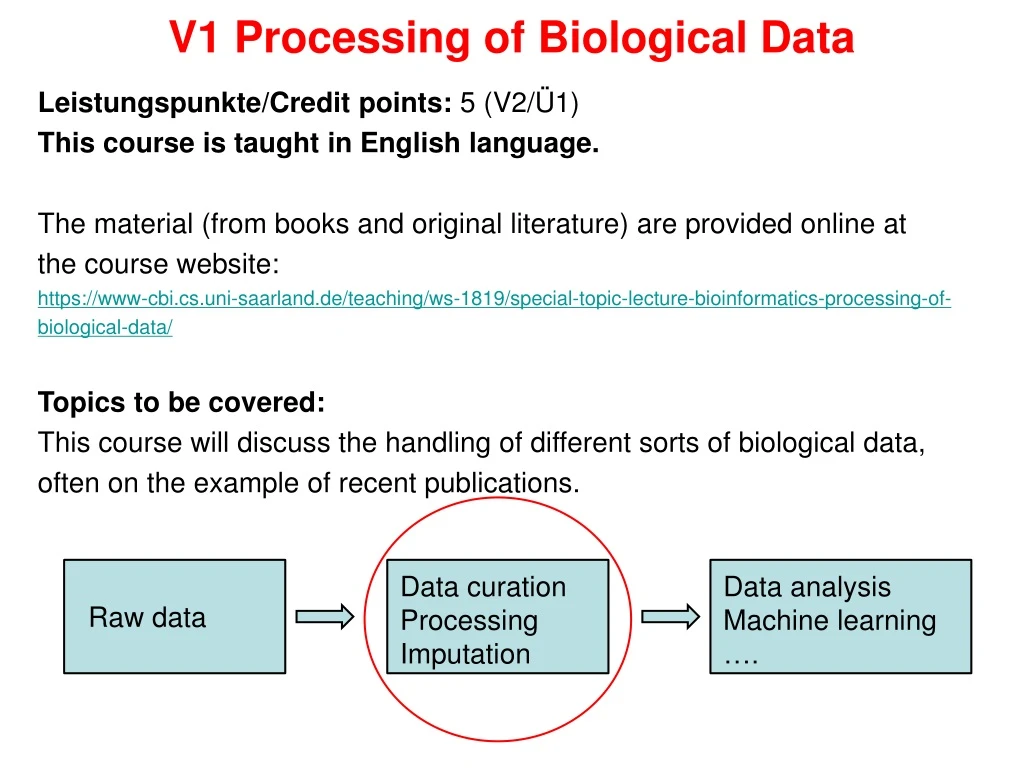
Leistungspunkte/Creditpoints: 5 (V2/Ü1) This courseistaught in English language. The material (frombooksand original literature) areprovided online at thecoursewebsite: https://www-cbi.cs.uni-saarland.de/teaching/ws-1819/special-topic-lecture-bioinformatics-processing-of-biological-data/ Topics tobecovered: This course will discussthehandlingof different sortsofbiologicaldata, often on theexampleofrecentpublications. V1 Processing of Biological Data Data curation Processing Imputation Data analysis Machinelearning …. Rawdata
We will handout 6 bi-weeklyassignments. Groups ofuptotwostudentscanhand in a solvedassignment. Send yoursolutionsbye-mailtotheresponsibletutors untilthetime+dateindicated on theassignmentsheet. The bi-weeklytutorialon Monday12.45 am – 2.15 pm (same room, time isnegotiable) will discusstheassignmentsolutions. On demand, thetutorsmay also givesomeadviceforsolvingthenewassignments. Tutorial
The successfulparticipation in thelecturecourse („Schein“) will becertified upon fulfilling • Schein condition 1 : ≥ 50% ofthepointsfortheassignments - Schein condition2 : pass final writtenexamat end ofsemester The grade on your „Schein“ will equalthatofyour final exam. Everybodywhotookthe final exam (andpasseditordid not pass it) andthosewhohavemissedthe final exam cantakethere-exam at thebeginningofWS17/18. Schein conditions
V1: bacterialdata (S. aureus): clustering / PCA (R. Akulenko) V2: bacterialdata/DNA methylation: predictionofmissingvalues (BEclear, R. Akulenko) V3: differential geneexpression, detectionofoutliers (A. Barghash) V4: MS proteomicdata, imputation, normalization (D. Nguyen), proteinarrays (M. Pedersen) V5: peakdetection, breathomics (AC Hauschild) V6: shapedetection, processingofkidneytumor MRI scans (Vera Bazhenova) V7: genomicsequences, SNPs (M. Hamed, K. Reuter, Ha Vu Tran) V8: functional GO annotations (M. Hamed, Ha Vu Tran) V9: curvefitting, datasmoothing (AKSmooth …) V10: protein X-raystructures: titrationstates, hydrationsites, multiple sidechainandligandconformations, superposition … protein-protein complexes: crystalcontacts, interfaces, … V11: analysisof MD simulationtrajectories: correlationofsnapshots, remove CMS motion V12: multi-variateanalysis V13: integrative analysisof multidimensional datasets (D. Gaidar, M. Nazarieh) Planned lecture - overview
Data preprocessingisoneofthemostcriticalsteps in datamining. Data preprocessingmethodsaredividedinto 4 categories: • Data cleaning • Data integration • Data transformation • Data reduction Data preprocessing Data Mining: KnowItAll byIan H. Wittenet al. Publisher: Morgan Kaufmann (2008)
◦ Data cleaning: fill in missing values, smooth noisy data, identify or remove outliers, and resolve inconsistencies. ◦ Data integration: using multiple databases, data cubes, or files. ◦ Data transformation: normalization and aggregation. ◦ Data reduction: reducing the volume but producing the same or similar analytical results. ◦ Data discretization: part of data reduction, replacing numerical attributes with nominal ones. Data preprocessing Data Mining: KnowItAll byIan H. Wittenet al. Publisher: Morgan Kaufmann (2008)
Data summarization: quantile plot Interpretation: Branch 2 has – on average – higherunitprices. Data Mining: KnowItAll byIan H. Wittenet al. Publisher: Morgan Kaufmann (2008)
Whole Genome SequenceTypingand MicroarrayProfilingofMethicillin-Resistant Staphylococcusaureusisolates • Classification of MSSA / MRSA S. aureus strains in Saarland (PLoS ONE 2012) • DFG Germany-Africa project (J. Clin. Microbiol. 2016; Sci. Reports 2017) • Co-workers • (1) RuslanAkulenko, Ulla Ruffing, Mathias Herrmann, Lutz von Müller, • (2) StaphNet Consortium led by Mathias Herrmann, funded by DFG
Pilot study: classification of resistant Staphylococcus aureus strains Aim: classify MRSA / MSSA accordingtogenerepertoire
any strain of S. aureuswith resistance to beta-lactam antibiotics: penicillins; cephalosporins; Need to classify MRSA strains to detect infections, prevent transmission Methycillin sensitive/resistant Staphylococcus aureus (MSSA/MRSA) MSSA MRSA anaerobic Gram-positive coccal bacterium, frequently part of the normal skin flora, 60% of population are carriers
DNA preparation of polymorphic X-region of staphylococcusprotein A from S. aureus (Spa) amplify by PCR sequencing assignment using RidomStaphType software routine: Characterize MRSA by Spa-typing
Results from Spa-typing: splits graph For MSSA, spa-typing allowed for good discrimination of patient isolates. However, the majority of MRSA isolates clustered into clonal complex CC5/t003. This hampers sub-classification by spa-typing Unroutedtreegeneratedwith www.splitstree.org MSSA strainslabeled S__ MRSA strainslabeled R__
DNA microarray (IdentiBAC – Alere) Microarraycontains 334 DNA probesfor genes/regionsthatareclinically relevant and/orrelevant forclonaltyping alere-technologies.com
DNA microarrayprinciple The extracted RNA free genomic DNA from the bacterial overnight culture is internally biotin labelled through a set of antisense primers. The resulting single stranded and biotin labelled amplicons are hybridized to a set of discriminative probes that are covalently bound onto the microarrays. The biotin labelled DNA bound to the probes on the array is subsequently stained. alere-technologies.com
Process microarray data (334 probes) Simple idea: Compute Euclidian distance between samples Other distances are possible, also weighted distances, where some probes get higher weights.
Hierarchical agglomerative clustering based on MA data MRSA MSSA Hierarchical clustering: (1) Calculate pairwise distance matrix for all samplesto be clustered. (2) Search distance matrix for two most similar samplesor clusters (initially each cluster consists of a single sample). If several pairs have the same separation distance, a predetermined rule is used to decide between alternatives. (3) The two selected clusters are merged to produce a new cluster that now contains at least two objects. (4) The distances are calculated between this new cluster and all other clusters. (5) Repeat steps 2–4 until all objects are in one cluster. Clustering based on EuclidiandistanceyieldsalmostperfectseparationbetweenMSSA/MRSA excepttheencircledresistantsamples
S. aureus in Germany vs. Africa: StaphNet 6 study sites each collected 100 isolates of healthy volunteers and 100 of blood culture or clinical infection sites → 1200 isolates Aim microbiological and molecular characterization of African S. aureus isolates by DNA microarray analysis including clonal complex analysis supplemented by Whole Genome Sequencing
Münster Freiburg Homburg Münster Freiburg Homburg Lambaréné Lambaréné Ifakara Ifakara Lambaréné Lambaréné Manhiça Manhiça What does the microarray measure? Naively, one can interpret the microarray result as 1 : gene is present in the strain 0 : gene is not present in the strain However, false negative non-detections of particular targets may occur due to non-binding of the sample amplicon to the microarray’s probe or primer oligonucleotide due topolymorphisms in the respective target gene. On the other hand, false positive results may occur between highly similar probe and amplicon sequences, e. g. between agrI and agrIV. → check MA results by whole genome sequencing Strauss et al. J ClinMicrobiol (2016) Bouaké Bouaké Bouaké Kinshasa Kinshasa Kinshasa
MA assignment to CCs confirmed by whole-genome sequencing 154 S. aureusisolates (182 target genes) from Germany-vs-Africastudy → 97% agreementof MA and WGS Strauss et al. J ClinMicrobiol (2016)
Distribution of clonal complexes Some clonal complexes (CC) are more prevalent in Africa, others predominant in Germany.
Imbalance of hybridizing resistance genes? OR: odds ratio ; ratio of events to non-events CI95 : confidence interval
Antibiotic resistance The majority of resistance genes were equally distributed among isolates from Africa and Germany. Striking differences in phenotypic resistance could be observed for tetracycline and trimethoprim-sulfamethoxazole with a larger proportion of resistant isolates in the African population, and clindamycin, with resistance more prevalent among German isolates
neighbor-joining tree based on the allelic profiles of 1861 S. aureus core genome features. -> the majority of clusters are based on the geographical region. Clusters of isolates from infection or colonization were not detected Phylogenetic tree based on WGS data of 154 strains
Can’t see too much Clustering of all 1200 microarray samples is not handy
Principle component analysis of 1200 strains Input data: binarymatrixof MA data; dimension 1200 x 334 probes PCA identifieslocalgeneclustersthatarecharacteristic forparticularclonalcomplexes Color code: 6 different sites Marked in boxes: Characteristicgenes present in thiscluster.
PCA- intro PCA is the most popular multivariate statistical technique. It is used by almost all scientific disciplines. It is likely also the oldest multivariate technique. Its origin can be traced back to Pearson, Cauchy, Jordan, Cayley etc This part of the lecture is based on the article “Principal component analysis” by Herve Abdi & Lynne J. Williams in WIREs Computational Statistics, 2, 433-459 (2010)
PCA- intro PCA analyzes a data table X representing observations described by several dependent variables, which are, in general, inter-correlated. The goal of PCA is to extract the important information from the data table and express this information as a set of new orthogonal variables called principal components. We will consider a data table XofI observations and J variables. The elements are xij. The matrix X has rank L where L min [I,J]
PCA- preprocessing data entries In general, the data table will be preprocessed before the analysis. The columns of X are centered so that the mean of each column is equal to 0. If in addition, each element of X is divided by or , the matrix = XTXis a covariance matrix, and the analysis is referred to as covariance PCA.
PCA- preprocessing data entries In addition to centering, when the variables are measured with different units, it is customary to standardize each variable to unit norm. This is obtained by dividing each variable by its norm (i.e. the square root of the sum of all squared elements of this variable) , which is equivalent to dividing it by its standard deviation (except dividing by n vs n-1). In this case, the analysis is referred to as a correlation PCA because, then, then matrix XTX is a correlation matrix. We will make use of the fact that the matrix X has a singular value decomposition (SVD) What is a SVD?
Insert: review of eigenvalues A vector u that satisfies A u = u or ( A - I )u = 0 is an eigenvector of this matrix A. The scalar value is the eigenvalue associated with this eigenvector. For example, the matrix has the eigenvectors with eigenvalue 1 = 4. Test 23 + 32 = 43; 2 3 + 1 2 = 4 2 and with eigenvalue 1 = -1. Test 2 (-1) + 3 1 = (-1) (-1) ; 2 (-1) + 1 1 = (-1) 1
Insert: review of eigenvalues For mostapplicationswenormalizetheeigenvectors so thattheirlengthisequalto 1, i.e. Traditionally, we put the set of eigenvectors of A in a matrix denoted by U. Then, each column of Ucontainsan eigenvector of A. The eigenvalues are stored as diagonal elements of a diagonal matrix . Then we can write A U = U or: A = U U-1(if we multiply with U-1) This is the eigendecomposition of this matrix. Not all matrices have a EDC.
Insert: positive (semi-) definite matrices A type ofmatricesusedoften in statisticsarecalledpositive semi-definite (PSD) The eigen-decompositionof such matricesalwaysexists, andhas a particularlyconvenient form. A matrix A is positive (semi-)definite, if there exists a real-valued matrix X and Correlation matrices, covariance, and cross-product matrices are all semi-definite matrices. The eigenvalues of PSD matrices are always positive or null. The eigenvectors of PSD are pairwise orthogonal when their eigenvalues are different.
Insert: positive (semi-) definite matrices This implies Then we can express A as with where U is the matrix storing the normalized eigenvectors. E.g. can be decomposed as = with showing that the 2 eigenvectors are orthonormal.
Singular Value Decomposition (SVD) SVD is a generalizationofthe eigen-decomposition. SVD decomposes a rectangularmatrixAintothree simple matrices: two orthogonal matricesPandQandone diagonal matrix. P : contains the normalized eigenvectors of the matrix . (i.e. The columns of P are called left singular vectors of A. Q : contains the normalized eigenvectors of the matrix . (i.e. The columns of Qare called right singular vectors of A. : the diagonal matrix of the singular values. They are the square root values of the eigenvalues of matrix (they are the same as those of ).
Interpretation of SVD In the special, yet common, case when M is an m × m real square matrix with positive determinant: U, V∗, and Σ are real m × m matrices as well. Σ can be regarded as a scaling matrix, and U, V∗ can be viewed as rotation matrices. www.wikipedia.org
Goals of PCA Extractthemostimportantinformationfromthedatatable →PC1 shoulddescribethedirectionalongwhichthedatacontainsthelargestvariance; PC2 is orthogonal to PC1 anddescribesthedirectionofthelargestremainingvarianceetc Compressthesizeofthedatasetbykeepingonlythisimportantinformation Simplifythedescriptionofthedataset Analyzethestructureoftheobservationandthe variables. In order to achieve these goals, PCA computes new variables called principal components (PCs) as linear combinations of the original variables. PC1 is the eigenvector of with largest eigenvalue etc.
PCA example PCA of a multivariate Gaussian distribution X centered at (1,3) with a standard deviation of 3 in roughly the (0.866, 0.5) direction and of 1 in the orthogonal direction. The two PCA vectors shown are the eigenvectors of the covariance matrix scaled by the square root of the corresponding eigenvalue, and shifted so that their tails are at the mean. Note thatshownhereisthedataalongthe original coordinates. In a PCA plot, thedataisprojectedontotwo PCs, usually PC1 and PC2. www.wikipedia.org
Deriving the components The principal components are obtained from the SVD of X, Q contains the principal components (normalized eigenvectors of ). The I x L matrix of factor scores, denoted F, is obtained as Thus, F can be interpreted as a projection matrix because multiplying X with Q gives the values of the projections of the observations X on the principal components Q.
PCA of MA hybridization data (again) PCA identifieslocalclustersthatarecharacteristic forparticularclonalcomplexes Projection (factor score) ofdatapoints on PC1
Summary • What we have covered today: • Detection of DNA probes by DNA microarray • Euclidian distance of 1/0 signals as distance measure • Clustering of MA data • PCA analysis of MA data Next lecture: - Reconstruct missing (ambiguous) data values with BEclear