Download
1 / 37
370 likes | 488 Vues
Perspectives on Climate Modeling Summer school-BNU-Beijing 5 Aug. 2006. Robert E. Dickinson Georgia Tech. Climate Model – what does it do?. Starts with known physical laws – conservation of momentum, energy, & mass.

E N D
Perspectives on Climate ModelingSummer school-BNU-Beijing 5 Aug. 2006 Robert E. Dickinson Georgia Tech
Climate Model – what does it do? • Starts with known physical laws – conservation of momentum, energy, & mass. • Views atmosphere, oceans, land as a continuum (i.e. all spatial scales present satisfying same laws). • Find and uses numerical approximations to the continuum physical laws. • Integrate in time to develop climate statistics same as observed-evaluate success by extent of agreement. • On global scale, this agenda very successful.
Climate Model Scaling/parameterization Need to describe details within the grid boxes
What limits success of climate models? • Processes occur on smaller scales that are different than those resolved on the larger scales. • These: a) affect the large scale rules b) change climate on scales that humans live on. • Have to some extent been recognized for long time – their inclusion has been called “parameterization” but better called “scaling”.
What is the problem? • Many of the practical aspects of climate modeling are centered at the land surface • Such modeling implicitly involves many spatial scaling issues, the more important ones may still be poorly represented; • issue of land coupling to precipitation, • limited by lacks in treatment of moist processes (convection, clouds, aerosol and cloud micro-physics, etc.).
Progression of Progress on this Topic. • Assume state variables on resolved scale: • Temperature, soil moisture, vegetation properties, • Homogeneous turbulent fluxes, uniform precipitation • Look for what not working because of excessive nonlinearity of processes. • Find ways to efficiently include missing effects with adequate realism and generality
Examples of processes needed to be parameterized and how first done. • Clouds and their effect on radiation and precipitation-put in as a fractional cover. • Prescribed from observations; then correlated with relative humidity. • Connections to precipitation neglected. • Precipitation and its connection to humidity. • All atmospheric water in excess of some “critical” relative humidty assumed converted to precipitation and moved to surface as rain or snow.
Other key examples of parameterization. • Boundary layer turbulence-how it exchanges momentum, heat, and moisture between surface and boundary layer, and free atmosphere? • How boundary layer processes connect to clouds and precipitation? • Collective effect of leaves and roots extract water from soil & move to atmosphere? • Moist convection – how make clouds & P?
Collective impact of “subgrid” processes • Dynamical model viewpoint :Q, external parameters, X = state variable; changes according to: d X/ dt = F(X,Q) (1) • X = [X] + X’ , the resolved and unresolved scales. Because of nonlinearities, to solve Eq.(1) for resolved scales, requires introducing some statistics of unresolved scales as additional degrees of freedom.
Climate is a Dynamic System Climate system responses Forces on Climate system IMPACTS Feedbacks Many processes on many scales change and modify the changing state
What has been done & what needed? • Have used simple conceptualizations of processes and with limited observations. • Now with more advanced computational and observational tools, can look much more carefully at details of processes and establish more elaborate and realistic relationships. • E.g. use cloud resolving and and large eddy resolving models. • Advanced field programs and satellite data
Observations very important • Local surface • Meteorological system • Field programs • Aircraft • Satellite • Requires international cooperation and sharing.
TOPEX/Poseidon Aqua SORCE QuikScat Sage TRMM SeaWinds Terra UARS Landsat 7 Grace Spaceborne Earth Observation Systems EO-1 SeaWiFS IceSat ACRIMSAT Toms-EP ERBS Jason
Land Scaling from Modeling Perspective • Climate model grid squares have sides of 100 km (within factor of 4 in either direction). • Land-surface model describes processes on spatial scale of about 10 m (“plot or point” scale”). • If scaling assumptions are made part of this description, scale dependent -easily lost in model revision. • e.g. Bonan (1996) LSM model – p 91-canopy evaporation limited to 20% of precipitation, left out of newer CLM.
Rules for Scaling to a Climate Model Plot scale Land-surface Model Global Data Sets Describing Land Interface to Atmospheric Model
Hydrological examples – impacts of scaling • Transpiration and soil evaporation depend nonlinearly on soil moisture. • What if 50% W = 0, and 50% W =1.0,versus W=0.5? ET 50% W
Leaf evaporation of intercepted precipitation. What if P = 0.5 mm/h over all grid-square versus 5 mm/h over 10% of grid square?
How precipitation changed if Tibet Plateau e.g. all at 4.7 km versus a distribution of elevations from 3 km to 6 km?
Current models Reality Thanks to B. Pinty for fig.
What changes if leaf area LAI = 3 of 100% versus 6 over 50% and 0 over 50%? • How can we average the z0 roughness of forest and grasland? • Such vegetation related averaging questionshandled by the widely used “Tiling” approach • Bin by plant types (pfts)+ barren, glacier, lake • Can assume either: • No competition for light, nutrients, water • Competition for water …(single soil column)
Issue of (Land) Complexity • Have a lot of little pieces (e.g. T’s or W’s) • Want to make them add up to one (or a few) pieces • View as a large number of dimensions – want to project to one (or a few) dimensions. • Commonly done by simple averaging of plots but for model may want more stringent physical requirements:
For reduction to low-dimensionality land model • Provide plausible two-way linkages to the large scale atmospheric variables. • Provide connections between the low-dimensional variables. • Maintain conservation of whatever is conserved – energy, moisture, …
Stochastic Viewpoint • An available tool for climate modeling • Science is what we see & efficient ways to summarize & use to infer what we have not seen. • Various forms of mathematics provide such summarizing tools • Climate model formulation has traditionally been deterministic, but has always used statistics for summarizing – and more sophisticated application are mostly recent, e.g. many papers using pdfs to help describe the formation of clouds.
Use of Distributions • If we want to average a function of some variable, f(P), where P here is precipitation, can’t simply put in an “average” P • Need to average f(P) using all the values of P that occur. • May be a lot of detail, but “histogram” summary statistic can provide all that is needed to do the average
Applied to land in climate model • Suppose N different values of P can occur • Can compute a separate land model for each value – we already do that for different points in space. • Can simply use one of the P’s – chosen randomly –stochastic (Monte Carlo) sampling – doing only one time probably worse than using the average P- but if done enough times, ends up sampling the distribution. • b) is more economical, but it cannot give the land the P made by the atmosphere - fatal
A major old but new issue • How are land processes and P coupled? • Depends on surface fluxes of heat and moisture (long-wave?) • Connects to heterogeneities in these fluxes (elevation, variations in vegetation, soil wetness) • Mediated through boundary layer – Jarvis McNaughton suggested BL damps impacts of vegetation.
qa2 Top of Boundary Layer We qa1 rc
What can be said? • AMIP II simulations – AHS study • GLACE intercomparisons: • Some of problem differences in land model • Some from differences in atmospheric model