Download
1 / 33
340 likes | 363 Vues
Delve into the impacts of climate change on ice sheets, including Antarctic and Greenland ice dynamics, sea level rise projections, and essential terms related to glaciers. Discover recent observations, expert opinions, and potential future scenarios.

E N D
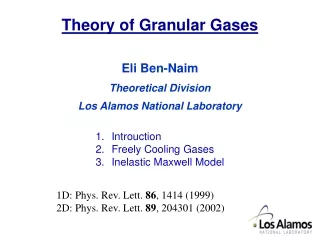
Ice Sheets and Climate Change William H. Lipscomb Los Alamos National Laboratory
What is an expert? “An expert is somebody who is more than 50 miles from home, has no responsibility for implementing the advice he gives, and shows slides.” Edwin Meese III
Acknowledgments • Jay Fein, NSF • DOE Office of Science • Phil Jones, LANL • Bill Collins, Bette Otto-Bleisner and Mariana Vertenstein, NCAR • Tony Payne and Ian Rutt, Univ. of Bristol • Jeff Ridley and Jonathan Gregory, UK Hadley Centre • Frank Pattyn, Free Univ. of Brussels • Slawek Tulaczyk, UC-Santa Cruz
Outline • Introduction to ice sheets • IPCC Third Assessment Report • Recent observations • Ice sheet models • Coupled climate-ice sheet modeling
Definitions • A glacieris a mass of ice, formed from compacted snow, flowing over land under the influence of gravity. • An ice sheet is a mass of glacier ice greater than 50,000 km2 (Antarctica, Greenland). • An ice cap is a mass of glacier ice smaller than 50,000 km2 (e.g., Svalbard). • An ice shelf is a large sheet of floating ice attached to land or a grounded ice sheet. • An ice stream is a region of relatively fast-flowing ice in a grounded ice sheet.
Antarctic ice sheet • Volume ~ 26 million km3 (~61 m sea level equivalent) • Area ~ 13 million km2 • Mean thickness ~ 2 km • Accumulation ~ 2000 km3/yr, balanced mostly by iceberg calving • Surface melting is negligible Antarctic ice thickness(British Antarctic Survey BEDMAP project)
East Antarctica (~55 m SLE) Grounded above sea level; not vulnerable to warming West Antarctica (~5 m SLE) Grounded largely below sea level; vulnerable to warming Antarctic peninsula (~0.3 m SLE) Mountain glaciers; may be vulnerable to warming Ice shelves Vulnerable to ocean warming; removal could speed up flow on ice sheet Antarctic regions Ice flow speed (Rignot and Thomas, 2002)
Volume ~ 2.8 million km3 (~7 m sea level equivalent) Area ~ 1.7 million km2 Mean thickness ~ 1.6 km Accumulation ~ 500 km3/yr Surface runoff ~ 300 km3/yr Iceberg calving ~ 200 km3/yr Greenland ice sheet Annual accumulation (Bales et al., 2001)
Global mean temperature was 1-2o higher than today Global sea level was 3-6 m higher Much of the Greenland ice sheet may have melted Eemian interglacial (~130 kyr ago) Greenland minimum extent(Cuffey and Marshall, 2000)
Last Glacial Maximum: ~21 kyr ago • Laurentide, Fennoscandian ice sheets covered Canada, northern Europe • Sea level ~120 m lower than today
Sea level change since Eemian IPCC TAR (2001), from Lambeck (1999) • Current rate of increase is ~18 cm/century • Past rates were up to 10 times greater
IPCC Third Assessment Report: Sea level change • Global mean sea level rose 10-20 cm during the 20th century, with a significant contribution from anthropogenic climate change. • Sea level will increase further in the 21st century, with ice sheets making a modest contribution of uncertain sign.
IPCC TAR: Stability of Greenland • “Models project that a local annual-average warming of larger than 3°C, sustained for millennia, would lead to virtually a complete melting of the Greenland ice sheet.” • This projection is based on standalone ice sheet models (Huybrechts & De Wolde, 1999; Greve, 2000). Positive feedbacks (elevation, albedo) speed melting. • Models also suggest that if Greenland were removed in present climate conditions, it would not regrow (Toniazzo et al., 2004). There may be a point of no return . . .
GCMs predict that under most scenarios (CO2 stabilizing at 450-1000 ppm), greenhouse gas concentrations by 2100 will be sufficient to raise Greenland temperatures above the melting threshold. IPCC scenarios and Greenland Greenland warming under IPCC forcing scenarios (Gregory et al., 2004)
Effect of 6 m sea level rise Florida; h < 6 m in green region Composite satellite image taken by Landsat Thematic Mapper, 30-m resolution, supplied by the Earth Satellite Corporation. Contour analysis courtesy of Stephen Leatherman.
IPCC TAR: Ice sheet dynamics • “A key question is whether ice-dynamical mechanisms could operate which would enhance ice discharge sufficiently to have an appreciable additional effect on sea level rise.” • Recent altimetry observations suggest that dynamic feedbacks are more important than previously believed.
Laser altimetry shows rapid thinning near Greenland coast: ~0.20 mm/yr SLE Thinning is in part a dynamic response: possibly basal sliding due to increased drainage of surface meltwater. Ice observed to accelerate during summer melt season (Zwally et al., 2002) Recent observations: Greenland Ice elevation change (Krabill et al., 2004)
Large glaciers (Pine Island, Thwaites, Smith) flowing into the Amundsen Sea are thinning, probably because of warm ocean water eroding ice shelves (Payne et al., 2004; Shepherd et al., 2004) Thinning extends ~200 km inland Sea level rise ~ 0.16 mm/yr from West Antarctic thinning Recent observations: West Antarctica Ice thinning rate (Shepherd et al., 2004)
Recent observations: Antarctic peninsula • Glaciers accelerated by up to a factor of 8 after the 2002 collapse of the Larsen B ice shelf (Scambos et al., 2004; Rignot et al., 2004) Oct. 2000 Dec. 2003 (Rignot et al., 2004)
SAR measurements suggest that East Antarctica is thickening by ~1.8 cm/yr , probably because of increased snowfall SLE ~ -0.12 mm/yr; could cancel out West Antarctic thinning Recent observations: East Antarctica Ice elevation change, 1992-2003 (Davis et al., 2005)
Slippery slope? • Ice sheets can respond more rapidly to climate change than previously believed. • We need to better understand the time scales and mechanisms of deglaciation. Photo by R. J. Braithwaite. From Science, vol. 297, July 12, 2002.
Upper boundary 1. Air temperature 2. Snowfall minus melt Ice flow 1. Gravity balanced locally 2. Glen’s flow law for horizontal velocity 3. Vertical velocity from flow divergence z Temperature evolution 1.Diffusion 2. Advection 3. Dissipation Thickness evolution 1. Horizontal flow divergence 2. Accumulation T Lower boundary 1. Slip velocity 2. Basal friction 3. Geothermal heat flux Thermomechanical ice sheet models Isostasy 1. Flexure in response to ice load 2. Mantle flow Courtesy of Tony Payne
Ice sheet dynamics Ice sheet: vertical shear stress • Ice sheet interior: Gravity balanced by basal drag • Ice shelves: No basal drag or vertical shear • Transition regions: Need to solve complex 3D elliptic equations—still a research problem (e.g., Pattyn, 2003) Ice stream, grounding line: mixture Ice shelf: lateral & normal stress Ub=0 Ub = Us 0 < Ub <Us Courtesyof Frank Pattyn
Ice sheet mass balance b = c + a c = accumulation a = ablation Two ways to compute ablation: • Positive degree-day • Surface energy balance (balance of radiative and turbulent fluxes) Accumulation and ablation as function of mean surface temperature
Coupling ice sheet models and GCMs Why couple? Why not just force ice sheet models offline with GCM output? • As an ice sheet retreats, the local climate changes, modifying the rate of retreat. • Ice sheet changes could alter other parts of the climate system, such as the thermohaline circulation. • Interactive ice sheets are needed to model glacial-interglacial transitions.
Time and spatial scales • Ice sheet spatial scales are short compared to typical climate model components: • 10-20 km resolution needed to resolve ice streams • Similar resolution needed to resolve steep topography near ice edge (for accurate ablation rates) • Ice sheet time scales are long: • Flow rates ~10 m/yr in interior, ~1 km/yr in ice streams • Typical dynamic time step ~ 1-10 yr • Response time ~ 104 yr • Cf. GCM scales: Dx ~ 100 km, Dt ~ 1 hr
Coupling ice sheet models and GCMs Degree day Temperature P - E Interpolate to ice sheet grid Surface energy balance SW, LW, Ta, qa, |u|, P GCM Dx ~ 100 km Dt ~ 1 hr ISM Dx ~ 20 km Dt ~ 1 yr Ice sheet extent Ice elevation Runoff Interpolate to GCM grid
Challenges: Model biases Problem: GCM temperature and precipitation may not be accurate enough to give realistic ice sheets. Solution: Apply model anomaly fields with an observed climatology. Caveat: The model may not have the correct sensitivity if its mean fields are wrong.
Challenges: Asynchronous coupling Problem: Fully coupled multi-millennial runs are not currently feasible. Solution: Couple the models asynchronously, e.g. 10 GCM years for every 100 ISM years. Caveat: May not conserve global water, may not give the ocean circulation enough time to adjust.
Coupled climate-ice sheet modeling • Ridley et al. (2005) coupled HadCM3 to a Greenland ice sheet model and ran for 3000 ISM years (~735 GCM years) with 4 x CO2. • After 3000 years, most of the Greenland ice sheet has melted. Sea level rise ~7 m, with max rate ~50 cm/century early in simulation. • Regional atmospheric feedbacks change melt rate.
SGER proposal • I will couple Glimmer, an ice sheet model, to CCSM. • Developed by Tony Payne and colleagues at the University of Bristol • Includes shelf/stream model, basal sliding, and iceberg calving • Designed for flexible coupling with climate models • Initial coupling will use a positive degree-day scheme. • Future versions could include a surface energy balance scheme and full 3D stresses.
Key questions • How fast will the Greenland and Antarctic ice sheets respond to climate change? • At what level of greenhouse gas concentrations are existing ice sheets unstable? • Can we model paleoclimate events such as glacial-interglacial transitions? • To what extent will ice sheet changes feed back on the climate?