IS-LM
IS-LM. The Basic Model of Macro. Learning Objections. Understand the construction of the IS curve and how it describes equilibrium in the goods market Understand the construction of the LM curve and how it describes equilibrium in the Money market

IS-LM
E N D
Presentation Transcript
IS-LM The Basic Model of Macro
Learning Objections • Understand the construction of the IS curve and how it describes equilibrium in the goods market • Understand the construction of the LM curve and how it describes equilibrium in the Money market • Understand simultaneous equilibrium in the Goods and Money markets • Use the model to analyse the effects of Fiscal and Monetary policy
INTRODUCTION • Earlier we identified a role for government policy: stabilizing Output near the full capacity or “natural” level • Model that show how economic shocks can arise and what we can do about them • In the simple model of the last section the equilibrium level of output • (a) can be influenced by fiscal policy (changes in G and T) • (b) is not necessarily at capacity, or full employment • This is because the assumptions of the model are very restrictive: • no role for money or interest rates • prices and wages are by assumption inflexible • This is clearly not very realistic • In the section we relax the first restriction and look at interest rates • Later we will add to the model and relax many of the restrictive assumptions
Basic Structure of Model • Divide the economy into three markets and study how the interact • Goods market – Demand side • The simple model of the last section • Money Market • could expand to include other assets • Balance of Payments • connect with rest of world • Mundell-Flemming Model – Nobel Prize • This is left to the next section of the course
Goods Market (IS) • Mankiw 11.2 • This encapsulates the simple model of the previous section • Goods Market Equilibrium • Aggregate Supply (AS) = Aggregate Demand (AD) • GDP=Income: Y • Aggregate demand (AD) • Equilibrium – Plans realised • AS=AD • Y=AD • Assume prices fixed • Big issue • Is it reasonable? • Is it true? • Empirical evidence that true in the Short Run
Just review: What are the sources of demand for produced goods? • AD=C+I+G+NX • Private consumption: C(Y, r, T, Wealth) • Private Investment: I(r, Y) • Government Cons & Inv : G • Exports-Imports: NX(Yf,e,Y)=0 (for now…) • Plans vs actual i.e. model behaviour • Can make the model as complicated as you like • Size and sign of effects
Equilibrium: AD=Y • Had this before: notice new notation “AD” for “PE” AS=AD=Y AD AD Y* Y
Example of Change in G • Assume all except consumption are fixed • “exogenous” • G increases AD2=C+I+G2+X-M AD AD1=C+I+G1+X-M Y
AD • Fiscal Policy and Multiplier AD2 AD1 Y1* Y2* Y
Think of other “shocks” that might effect the economy in the same way • Fall in interest rates • Fall in taxes • Rise in world income • Increase in private investment (FDI) • A depreciation in the exchange rate (next section)
The effect of shock is larger than its size • More than one for one • Y=fn(C) and C=fn(Y) • Example: • Y=C+I+G • C=a+b(Y-T) a>0 0<b<1 • Y=a+b(Y-T)+I+G
Why is Multiplier>1 • Initial change in government expenditure: DG • Implies a change in income for some group: DY1= DG • This leads to a increase in their consumption DC1= bDY1= bDG • This in turn leads to a further increase in Y representing income for some other group DY2= DC1= bDG • This leads to another increase in consumption • DC2= bDY2= b(bDG)=b2DG
This leads to another round of income increase • The process continues for an infinite number of rounds • Total change in income • DY= DY1 +DY2 +…+ DYn+… • DYn=bn-1DG • DY= DG*[1+b+b2+…+bn-1+…] • DY= DG*[1/(1-b)] • Warning FP not a panacea • This is very simple model
IS: Output and Interest Rates • Split variables that can effect Y • endogenous : r (we will explain it later) • Exogenous: all others e.g. G, I, T • What happens when interest rates fall? • Output rises: consume and invest more • Plot a graph of all the interest rates and the associated Y from goods market • Locus of Goods Market Equilibrium • IS Curve i
Reduce interest rate • Consumption and investment rise for every level of income • Result is higher eqm income
AD AD2 AD1 Y Stability? r IS Y
Maths • Aside: Investment=Savings
THE IS-CURVE & Eqm • The IS-curve is the locus of all combinations of r and Y consistent with goods-market equilibrium • Plans are consistent • When out of equilibrium forces exit to pull the economy towards equilibrium r Y > Ye Y < Ye IS Y
What makes it Eqm? • If not on IS curve then we are not in equilibrium • Plans not being realised so something will change • We assume production adjusts • If Y<AD then production will increase • If Y>AD then production will fall • Note this is an assumption • This is a very simple model of AS • AS adjusts to meet whatever is demanded • Prices do not adjust • Counter intuitive to some but empirically accurate
SLOPE OF THE IS-CURVE • From The Equation of the IS curve we see that its slope is negative. • Note, the more I (or Consumption, etc) is responsive to changes in r, the larger is lambda • This in turn implies a lower slope coefficient (flatter IS curve) • Similarly, the less responsive I (or C or any element of AD) is to r , the steeper is the IS-curve. • Imagine you can control the economy by choosing r
SLOPE OF THE IS-CURVE • IS1 is more elastic: AD relatively responsive to changes in r • IS2 is less elastic: AD relatively un responsive to changes in r r IS2 IS1 0 Y
Hint about Curves • In economics in general for any curve you will need to understand two things • What determines the slope of the curve? • What causes the curve to shift ? • The answer to Q1 is usually “behavioral parameters” • E.g. the responsiveness of I to r; MPC • The answer to Q2 is “exogenous” variables • Often policy variables e.g. G
Movements of the Curve • Movements • in r represent movements along the IS curve. • Changes in other variables represent a parallel shift in IS e.g. change in G DY=mult*DG AD AD1 r DG AD2 IS2 IS1 Y Y
SHIFTS OF THE IS-CURVE • Outward shift: IS1to IS2 when G is > 0: Fiscal expansion • Trick to analyzing policy effects r IS2 IS1 0 Y
Money Market (LM) • Mankiw 11.2 • People have a demand for money • Liquidity preference: Money vs. Bonds • Money : cash, current accounts, demand deposits, little or no interest • Bonds: proxy for any asset with a return • Exact split is ambiguous • Why money at all? Transactions • Demand for liquidity increases as interest rate falls • Notation: “M” or “L” • Mankiw uses M/P but same as M as P is assumed fixed (for now)
A change in either M or r leads to a movement along the demand for money curve • An change in Y leads to a shift in the curve • Transactions demand
r L(Y2,r) L(Y1,r) M
Money supply is fixed by central bank • More on this later • For the moment think of open market operations • CB buys/sell bonds on open markets • Any asset in principle but almost always gov bonds • Uses cash or cheques drawn on itself • Buying bonds: Money supply rises • Selling bonds: Money supply falls
Effectively Money supply is exogenous • i.e. not a function of r or Y • Central bank preferences (a later topic) M r L M
What is the effect of an increase in Money supply? • Interest rates fall M1 M2 r L(r,Y) M
What about an increase in GDP • More transactions so interest rates rise M r L2 L1 M
Money Market Equilibrium • When Y increases Lincreases. Given Mthis leads to an excess demand for money, so r increases to r2 • For any given increase in y, by how much will r have to increase to restore equilibrium between Msand Md? • The depends on how responsive Lis to changes in r • The higher the interest-elasticity of the demand for Money, the smaller the increase in r necessary to restore equilibrium • As is usual equilibrium occurs if and only if all plans are consistent • How does this work here? • Interest rates adjust • Note logical inconsistency between adjustable interest rates and but fixed prices • Flexibility of financial vs goods markets • Empirically justified
LM: Output and Interest rates • As for IS, we split variables that can effect r • endogenous : Y • Exogenous: M • What happens when output fall? • Interest rate falls: seen this already • Plot a graph of all the interest rates and the associated Y from money market • Locus of Money Market Equilibrium • LM Curve
Reduce G • Income falls for every level of interest rate and money demand falls with it • Result is lower eqm interest rate
Ms/P LM r r L2 L1 Y M
Slope of LM Curve • Depends on the size of L2 vs L1 • L2 is sensitivity of money demand to interest rates • L1 is sensitivity of money demand to income • If l1 is really high would get a steeper LM curve as require only a very small increase in r after an increase in Y • L2 very high then get flatter LM
Movements • Movements in y represent movements along the LM curve. • Changes in other variables represent shift in LM Ms1 Ms2 LM1 r r LM2 L Y M
SHIFTS OF THE LM-CURVE (2) • The Central Bank (ECB, Federal Reserve, Bank of England….) is the main agent for implementing monetary policy • The CB can expand the Money Supply by Open Market purchases of bonds: this adds to Banks’ reserves and enables them to expand lending, etc. • Similarly, Open Market bond sales can leas to a fall in Ms • The CB can also change the rate at which it is prepared to lend to banks (Refinancing Rate, Federal Funds rate, REPO rate,…) • This impacts on the cost of funds to banks and therefore on the rates which they charge borrowers. It may also influence the amount of liquid reserve assets which banks wish to hold and therefore their willingness to expand credit, etc. • More about the details of monetary policy later.
SHIFTS OF THE LM-CURVE (3) • Suppose the Central Bank expandsM • This leads to excess of Ms over Md • Result: equilibrium r falls • The immediate effect is to displace the combination of (r, y) consistent with monetary equilibrium downwards • This corresponds to a rightwards (or downwards) shift in the LM curve • But will the fall in r lead to an increase in Aggregate Demand and therefore in y? • It will, and therefore we have to turn again to the IS-curve and the interaction between IS and LM.
IS & LM together • Both markets are linked • Both imply a link between Y and r • Money: Y -> Md-> r • Goods: r-> I-> Y • The intersection of the two curves gives the equilibrium • Jointly determines Y and r • For any policy or shock, • work out which exogenous variable moves • Which curve moves • New intersection is equilibrium
IS and LM • At E, there is both goods market and monetary equilibrium • Understand the forces bringing economy to equilibrium r LM Y >AD Md < Ms Y > AD Md > Ms Y < AD Md < Ms E Y < AD Md > Ms IS 0 y