PARAMETRIC EQUATIONS AND POLAR COORDINATES
10. PARAMETRIC EQUATIONS AND POLAR COORDINATES. PARAMETRIC EQUATIONS & POLAR COORDINATES. In Section 10.5, we defined the parabola in terms of a focus and directrix. However, we defined the ellipse and hyperbola in terms of two foci. PARAMETRIC EQUATIONS & POLAR COORDINATES.


PARAMETRIC EQUATIONS AND POLAR COORDINATES
E N D
Presentation Transcript
10 PARAMETRIC EQUATIONS AND POLAR COORDINATES
PARAMETRIC EQUATIONS & POLAR COORDINATES In Section 10.5, we defined the parabola in terms of a focus and directrix. However, we defined the ellipse and hyperbola in terms of two foci.
PARAMETRIC EQUATIONS & POLAR COORDINATES 10.6Conic Sections in Polar Coordinates In this section, we will: Define the parabola, ellipse, and hyperbola all in terms of a focus and directrix.
CONIC SECTIONS IN POLAR COORDINATES If we place the focus at the origin, then a conic section has a simple polar equation. • This provides a convenient description of the motion of planets, satellites, and comets.
CONIC SECTIONS Theorem 1 Let F be a fixed point (called the focus) and l be a fixed line (called the directrix) in a plane. Let e be a fixed positive number (called the eccentricity.)
CONIC SECTIONS Theorem 1 The set of all points P in the plane such that (that is, the ratio of the distance from Fto the distance from l is the constant e) is a conic section.
CONIC SECTIONS Theorem 1 The conic is: • an ellipse if e < 1. • a parabola if e = 1. • a hyperbola if e > 1.
CONIC SECTIONS Proof Notice that if the eccentricity is e = 1, then |PF| = |Pl| • Hence, the given condition simply becomes the definition of a parabola as given in Section 10.5
CONIC SECTIONS Proof Let us place the focus F at the origin and the directrix parallel to the y-axis and d units to the right.
CONIC SECTIONS Proof Thus, the directrix has equation x = dand is perpendicular to the polar axis.
CONIC SECTIONS Proof If the point P has polar coordinates (r, θ), we see that: |PF| = r |Pl| = d – r cos θ
CONIC SECTIONS Proof—Equation 2 Thus, the condition |PF| / |Pl| = e, or |PF| = e|Pl|, becomes: r = e(d – r cos θ)
CONIC SECTIONS Proof Squaring both sides of the polar equation and convert to rectangular coordinates, we get x2 + y2 = e2(d – x)2 = e2(d2 – 2dx + x2) or (1 – e2)x2 + 2de2x + y2 = e2d2
CONIC SECTIONS Proof—Equation 3 After completing the square, we have:
CONIC SECTIONS Proof If e < 1, we recognize Equation 3 as the equation of an ellipse.
CONIC SECTIONS Proof—Equations 4 In fact, it is of the form where
CONIC SECTIONS Proof—Equation 5 In Section 10.5, we found that the foci of an ellipse are at a distance c from the center, where
CONIC SECTIONS Proof This shows that Also, it confirms that the focus as defined in Theorem 1 means the same as the focus defined in Section 10.5
CONIC SECTIONS Proof It also follows from Equations 4 and 5 that the eccentricity is given by: If e > 1, then 1 – e2 < 0 and we see that Equation 3 represents a hyperbola.
CONIC SECTIONS Proof Just as we did before, we could rewrite Equation 3 in the form Thus, we see that:
CONIC SECTIONS By solving Equation 2 for r, we see that the polar equation of the conic shown here can be written as:
CONIC SECTIONS If the directrix is chosen to be to the left of the focus as x = –d, or parallel to the polar axis as y = ±d, then the polar equation of the conic is given by the following theorem.
CONIC SECTIONS Theorem 6 A polar equation of the form represents a conic section with eccentricity e. The conic is: • An ellipse if e < 1. • A parabola if e = 1. • A hyperbola if e > 1.
CONIC SECTIONS Theorem 6 The theorem is illustrated here. .
CONIC SECTIONS Example 1 Find a polar equation for a parabola that has its focus at the origin and whose directrix is the line y = –6.
CONIC SECTIONS Example 1 Using Theorem 6 with e = 1 and d = 6, and using part (d) of the earlier figure, we see that the equation of the parabola is:
CONIC SECTIONS Example 2 A conic is given by the polar equation • Find the eccentricity. • Identify the conic. • Locate the directrix. • Sketch the conic.
CONIC SECTIONS Example 2 Dividing numerator and denominator by 3, we write the equation as: • From Theorem 6, we see that this represents an ellipse with e = 2/3.
CONIC SECTIONS Example 2 Since ed = 10/3, we have: • So, the directrix has Cartesian equation x = –5.
CONIC SECTIONS Example 2 When θ = 0, r = 10. When θ = π, r = 2. • Thus, the vertices have polar coordinates (10, 0) and (2, π).
CONIC SECTIONS Example 2 The ellipse is sketched here.
CONIC SECTIONS Example 3 Sketch the conic • Writing the equation in the formwe see that the eccentricity is e = 2. • Thus, the equation represents a hyperbola.
CONIC SECTIONS Example 3 • Since ed = 6, d = 3 and the directrix has equation y = 3. • The vertices occur when θ = π/2 and 3π/2; so, they are (2, π/2) and (–6, 3π/2) = (6, π/2).
CONIC SECTIONS Example 3 It is also useful to plot the x-intercepts. • These occur when θ = 0, π. • Inboth cases, r = 6.
CONIC SECTIONS Example 3 For additional accuracy, we could draw the asymptotes. • Note that r→ ±∞ when 1 + 2 sin θ→ 0+ or 0- and 1 + 2 sin θ = 0 when sin θ=–½. • Thus, the asymptotes are parallel to the rays θ = 7π/6 and θ = 11π/6.
CONIC SECTIONS Example 3 The hyperbola is sketched here.
CONIC SECTIONS When rotating conic sections, we find it much more convenient to use polar equations than Cartesian equations. • We use the fact (Exercise 77 in Section 10.3) that the graph of r = f(θ – α) is the graph of r = f(θ) rotated counterclockwise about the origin through an angle α.
CONIC SECTIONS Example 4 If the ellipse of Example 2 is rotated through an angle π/4 about the origin, find a polar equation and graph the resulting ellipse.
CONIC SECTIONS Example 4 We get the equation of the rotated ellipse by replacing θwith θ – π/4 in the equation given in Example 2. • So, the new equation is:
CONIC SECTIONS Example 4 We use the equation to graph the rotated ellipse here. • Notice that the ellipse has been rotated about its left focus.
EFFECT OF ECCENTRICITY Here, we use a computer to sketch a number of conics to demonstrate the effect of varying the eccentricity e.
EFFECT OF ECCENTRICITY Notice that: • When e is close to 0, the ellipse is nearly circular. • As e→ 1-, it becomes more elongated.
EFFECT OF ECCENTRICITY When e = 1, of course, the conic is a parabola.
KEPLER’S LAWS In 1609, the German mathematician and astronomer Johannes Kepler, on the basis of huge amounts of astronomical data, published the following three laws of planetary motion.
KEPLER’S FIRST LAW A planet revolves around the sun in an elliptical orbit with the sun at one focus.
KEPLER’S SECOND LAW The line joining the sun to a planet sweeps out equal areas in equal times.
KEPLER’S THIRD LAW The square of the period of revolution of a planet is proportional to the cube of the length of the major axis of its orbit.
KEPLER’S LAWS Kepler formulated his laws in terms of the motion of planets around the sun. • However, they apply equally well to the motion of moons, comets, satellites, and other bodies that orbit subject to a single gravitational force.
KEPLER’S LAWS In Section 13.4, we will show how to deduce Kepler’s Laws from Newton’s Laws.
KEPLER’S LAWS Here, we use Kepler’s First Law, together with the polar equation of an ellipse, to calculate quantities of interest in astronomy.