Enhancing Arc Consistency with Algorithm AC-6: Efficient Initialization and Propagation
Algorithm AC-6 improves upon AC-4 by simplifying the maintenance of arc consistency in constraint networks. Instead of counting all supporting values, AC-6 only retains the lowest supporting value for each pair, streamlining both initialization and propagation phases. This results in reduced space complexity to O(ad), using singletons for supporting sets and maintaining essential data structures from AC-4. While the time complexity remains at O(ad²), AC-6 offers more efficient processing, making it suitable for handling various constraint satisfaction problems, including commonly studied benchmarks.

Enhancing Arc Consistency with Algorithm AC-6: Efficient Initialization and Propagation
E N D
Presentation Transcript
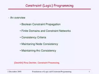
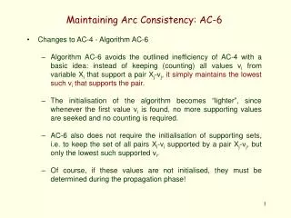
Maintaining Arc Consistency: AC-6 • Changes to AC-4 - Algorithm AC-6 • Algorithm AC-6 avoids the outlined inefficiency of AC-4 with a basic idea: instead of keeping (counting) all values vi from variable Xi that support a pair Xj-vj, it simply maintains the lowest such vi that supports the pair. • The initialisation of the algorithm becomes “lighter”, since whenever the first value vi is found, no more supporting values are seeked and no counting is required. • AC-6 also does not require the initialisation of supporting sets, i.e. to keep the set of all pairs Xi-vi supported by a pair Xj-vj, but only the lowest such supported vi. • Of course, if these values are not initialised, they must be determined during the propagation phase!
Maintaining Arc Consistency: AC-6 • Data Structures of Algorithm AC-6 • The List and the Boolean matrix M from AC-4 are kept. • The AC-4 counters are disposed of; • The supporting sets become “singletons”, keeping only the lowest value supported (it is assumed that some ordering is defined for the domains) sup(2,X1) = [X2-4,X3-1,X3-3,X4-1,X4-3,X4-4] % X1-2 supports(no attack) X2-4, X3-1,... sup(1,X1) = [X2-2, X2-3 , X3-2, X3-4, X4-2, X4-3] sup(3,X1) = [X2-1, X3-2 , X3-4, X4-1, X4-2, X4-4] sup(4,X1) = [X2-1, X2-2 , X3-1, X3-3, X4-2, X4-3]
Maintaining Arc Consistency: AC-6 • Both phases of AC-6 use predicate next_support(Xi,vi,Xj,vj, out v) that succeeds if there is in the domain of Xja “next” supporting value v, the lowest value, no less than some value, vj, such that Xj-v supports Xi-vi. predicate next_support(Xi,vi,Xj,vj, out v): boolean; sup_s <- false; v <- vj; while not sup_s and v =< max(dom(Xj))do if not satisfies({Xi-vi,Xj-v},Cij) then v <- next(v,dom(Xj)) else sup_s <- true end if end while next_support <- sup_s; end predicate.
Maintaining Arc Consistency: AC-6 • Algorithm AC-6 (Phase 1 - Inicialisation) procedure inicialise_AC-6(V,D,C); List <- ; M <- 0; sup <- ; for Cij in Cdo for vi in dom(Xi) do v = min(dom(Xj)) if next_support(Xi,vi,Xj,v,vj) then sup(vi,Xi)<- sup(vi,Xi) {Xj-vj} else dom(Xi) <- dom(Xi)\{vi}; M[Xi,vi] <- 0; List <- List {Xi-vi} end if end for end for end procedure
Maintaining Arc Consistency: AC-6 Algorithm AC-6 (Phase 1 - Inicialisation) procedure propagate_AC-6(V,D,C); while List do List <- List\{Xj-vj} % removes Xj-vj from List for Xi-vi in sup(vj,Xj) do sup(vi,Xi)<- sup(vi,Xi) \ {Xj-vj}; ifM[Xi,vi] = 1 then if next_suport(Xi,vi,Xj,vj,v) then sup(v,Xj)<- sup(v,Xj) {Xi-vi} else dom(Xi) <- dom(Xi)\{vi}; M[Xi,vi] <- 0; List <- List {Xi-vi} end if end if end for end while end procedure
Maintaining Arc Consistency: AC-6 • Space Complexity of AC-6 • In total, algorithm AC-6 maintains • Supporting Sets: In the worst case, for each of the a constraints Cij, each of the d pairs Xi-vi is supported by a single value vj form Xj (and vice-versa). Thus, the space required by the supporting sets is O(ad). • List: Includes at most 2a arcs • Matrix M: Maintains nd Booleans. • The space required by the supporting sets is dominant, so algorithm AC-6 has a space complexity of • O(ad) • between those of AC-3 ( O(a) ) and AC-4 ( O(ad2) ).
Maintaining Arc Consistency: AC-6 • Time Complexity of AC-6 • In both phases of initialisation and propagation, AC-6 executes next_support(Xi,vi,Xj,vj,v) in its inner cycle. • For each pair Xi-vi, variable Xj is checked at most d times. • For each arc corresponding to a constraint Cij, d pairs Xi-vi are considered at most. • Since there are 2a arcs (2 per constraint Cij), the time complexity, worst-case, in any phase of AC-6 is • O(ad2). • Like in AC-4, this is optimal assymptotically.
Maintaining Arc Consistency: AC-6 • Typical complexity of AC-6 • The worst case time complexity that can be inferred from the algorithms do not give a precise idea of their average behaviour in typical situations. • For such study, one usually tests the algorithms in a set of “benchmarks”, i.e. problems that are supposedly representative of everyday situations. • For these algorithms, either the benchmarks are instances of well known problems (e.g. N queens), or one relies on randomly generated instances parameterised by • their size (number of variables and cardinality of the domains) ; and • their difficulty (density and tightness of the constraint network).
Maintaining Arc Consistency: AC-6 Typical Complexity of algorithms AC-3, AC-4 e AC-6 (N-queens) # queens
Maintaining Arc Consistency: AC-6 Typical Complexity of algorithms AC-3, AC-4 e AC-6 (randomly generated problems) n = 12 variables, d= 16 values, density = 50% Tightness (%)
Maintaining Arc Consistency: AC-7 • Pitfalls of AC-6 - Algorithm AC-7 • Algorithm AC-6 (like AC-4 and AC-3) unnecessarily duplicates support detection, as it does not take into account that support is bidirectional, i.e. • Xi-vi supports Xj-vj iff Xj-vj supports Xi-vi • Algorithm AC-7 will use this property to infer support, rather than search for support. • Other types of inference could be used (for example, if one knows the semantics of the constraints, namely whether they are transitive), but AC-7 simply exploits the bidirectionality of support, which is always valid.
AC-3 8 tests AC-4 18 tests AC-6 8 tests AC-7 5 tests 2 inferences Maintaining Arc Consistency: AC-7 • Example: • Assuming that 2 countries may be coloured with 3 colours. The different AC-x algorithms will perform the following operation to initialise arc-consistency.
Maintaining Arc Consistency: AC-7 • Data Structures of Algorithm AC-7 • Algorithm AC-7 keeps, for each pair Xi-vi a supporting set CS(vi,Xi,Xj), that is the set of values from the domain of Xjcurrentlysupported by pair Xi-vi. • It also keeps, for each triple (vi,Xi,Xj), a value last(vi,Xi,Xj) that represents the last value (in increasing order) from the domain of Xj that was tested for support of pair Xi-vi. • For all variables, it is assumed that the domains have an ordering and, for convenience, artificial values top and bottom are added, respectively higher and lower that any “real” value of the domain.
Phase-1 of AC-7 • Algorithm AC-7 (Phase 1 - Inicialisation) • procedure inicialise_AC-7(V,D,C out Rem); • Rem <- ; • for Cij C and vi dom(Xi) do • CS(vi,Xi,Xj) <- ; last(vi,Xi,Xj) <- bottom; • end for • for Xi Vdo • forvi dom(Xi) do • for Xj | Cij C do • v <- seek_support(vi,Xi,Xj); • if v top then • CS(v,Xj,Xi) <- CS(v,Xj,Xi) {vi} • else • dom(Xi) <- dom(Xi)\{vi}; • Rem <- Rem {Xi-vi} • end if • end for • end for • end for • end procedure
Phase-2 of AC-7 • Algorithm AC-7 (Phase 2 - Propagation) • procedure propagate_AC-7(V,D,C,Rem); • while Rem do • Rem <- Rem \ {Xj-vj} • for Xi | Cij C do • while CS(vj,Xj,Xi) do • CS(vj,Xj,Xi) <- CS(vj,Xj,Xi) \ {vi} • if vi dom(Xi) then • v <- seek_support(vi,Xi,Xj); • if v top then • CS(v,Xj,Xi) <- CS(v,Xj,Xi) {vi} • else • dom(Xi) <- dom(Xi)\{vi}; • Rem <- Rem {Xi-vi} • end if • end if • end while • end for • end while • end procedure
Maintaining Arc Consistency: AC-7 • Algorithm AC-7 (Auxiliary Function seek_support) • Function seek_support seeks, within the domain of Xj, some value vj that supports pair Xi-vi. Firstly, it tries to infer such support in the pairs Xi-vi that support Xj-vj (exploiting the bidireccionality of support). Otherwise, it searches for vjin the domain of Xj in the usual way. • function seek_support(vi,Xi,Xj): value; • if infer_support(vi,Xi,Xj,v) then • seek_support <- v; • else • seek_support <-search_support(vi,Xi,Xj) • end if • end function • Notice that functions search_supportand seek_support may return the “artificial” value top.
Maintaining Arc Consistency: AC-7 • Algorithm AC-7 (Auxiliary Predicate infer_support) • Exploiting the bidireccionality of support, the auxiliary predicate infer_support, looks for a value vj in the domain of variable Xjthat supports pair Xi-vi. • predicate infer_support(vi,Xi,Xj,out vj): boolean; • found <- false; • while CS(vi,Xi,Xj) and not found do • CS(vi,Xi,Xj) = {v} Z; • if v in dom(Xj) then • found <- true; vj <- v; • else • CS(vi,Xi,Xj) = CS(vi,Xi,Xj) \ {v}; • end if • end do • infer_support <- found • end predicate.
Maintaining Arc Consistency: AC-7 • Algorithm AC-7 (Auxiliary Function search_support) • function search_support(vi,Xi,Xj): value; • b <- last(vi,Xi,Xj); • if b = top thensearch_support <- b • else • found <- false; b <- next(b,dom(Xj)) • while b top and not found do • if last(b,Xj,Xi) =< viand • satisfies({Xi-vi,Xj-b}, Cij) then • found <- true • else • b <- next(b,dom(Xj)) • end if • end while • last(vi,Xi,Xj) <- b; • search_support <- b; • end if • end function;
Maintaining Arc Consistency: AC-7 • Space Complexity of algorithm AC-7 • In total algorithm AC-7 maintains • Supporting Sets CS(vi,Xi,Xj): Like in AC-6, for each of the a constraints in C, and for each of the d pairs Xi-vi, it has a single value vj from the domain of Xj (that is supported by Xi-vi (and vice-versa). Hence, the space required by the supporting sets is O(ad). • Values last(vi,Xi,Xj): Identical • The space required by these structures dominates, so like AC-6, algorithm AC-7 possesses space complexity • O(ad) • between those of AC-3 (O(a)) and AC-4 (O(ad2)).
Maintaining Arc Consistency: AC-7 • Time Complexity of algorithm AC-7 • In both phases of initialisation and propagation, AC-7 executes seek_support(vi,Xi,Xj) in its inner cycle. • There are at most 2ad triples (vi,Xi,Xj), since there are 2a arcs corresponding to constraints in C, and the domain of each variable has, at most, d values. • In each call to seek_support(vi,Xi,Xj),d values from the domain of Xj, at most, are tested. • Hence, the worst-case time complexity of both phases of AC-7, is similar to that of AC-6, namely • O(ad2). • which, as shown with AC-4, is assymptotically optimal.
Maintaining Arc Consistency: AC-7 • Given their identical complexity, in what ways does AC-7 improve on AC-6 (and other AC-x algorithms)? Let us consider some features of AC-7. • It never tests Cij(vi,vj) if there is a v’j still in the domain of Xjsuch that Cij(vi, v’j) was successfully tested. • It never tests Cij(vi,vj) if • It has already been tested; or • If Cij(vj,vi) was already tested. • It has space complexity O(ad) • In contrast, algorithm AC-3 only exhibits feature 3; AC-4 only feature 2a; and AC-6 exhibits features 1, 2a and 3, but not feature 2b.
Maintaining Arc Consistency: AC-7 • Typical complexity of AC-6 • These feautures cannot be detected in worst case complexity analysis, that does not show any differences between algorithms AC-6 and AC-7. • The next results consider ramdomly generated problems with the parameters shown in the table below. The first ones are “easy” (under- and over-constrained). The last two lie in the phase transition, and the consistent (a) and inconsistent (b) instances are shown separately.
Maintaining Arc Consistency: AC-7 Comparison of Typical Complexity (#of checks)
Maintaining Arc Consistency: AC-7 Comparison of Typical Complexity (CPU time, in ms, in a Pentium at 200 MHz)
Maintaining Arc Consistency: AC-3d Bidirectionality of support was also exploited in an adaptation, not of AC-6, but rather of AC-3, resulting in algorithm A-3d. The main difference between algorithms AC-3 and AC-3d consists of the fact that whenever arc aijis removed from queue Q, the arc aji is also removed, in case it is there. In this case, both domains of Xi and Xjare revised, which avoids much duplicated work. Although it does not improve the worst-case complexity of AC-3, the typical complexity of AC-3d seems quite interesting (namely in some problems for which extensive tests were performed).
Maintaining Arc Consistency: AC-3d Comparison of Typical Complexity (# of checks) (previous ramdomly generated problems)
Maintaining Arc Consistency: AC-3d Comparison of Typical Complexity (previous ramdomly generated problems) (equivalent CPU time, in ms, in a Pentium at 200 MHz)
Maintaining Arc Consistency: AC-3d Results seem particularly interesting for problems in which AC-7 was proved much superior to AC-6, both in number of tests and in CPU time. This is the case of problem RLFAP (Radio Link Frequency Assignment Problem), that consists of assigning radio frequencies in a safe way (no risk of scrambling), for which instances with 3, 5, 8 e 11 antenae were studied. The code ( as well as that of other benchmark problems) may be found in a benchmark archive, available from the internet, in URL http://ftp.cs.unh.edu/pub/csp/archive/code/benchmarks
Maintaining Arc Consistency: AC-3d Comparison of Typical Complexity (# of checks) (RFLAP problems)
Maintaining Arc Consistency: AC-3d Comparison of Typical Complexity (RFLAP problems) (equivalent CPU time, in ms, in a Pentium at 200 MHz)
Path Consistency In addition to arc consistency, other types of consistency may be defined for binary constraint networks. Path consistency is a “classical” type of consistency, stronger than arc consistency. The basic idea of path consistency is that, in addition to check support in the arcs of the constraint network between variables Xi and Xj, further support must be checked in the variables Xk1, Xk2... Xkm that form a path between Xi and Xj, i.e. whenever there are constraints Ci,k1, Ck1,k2, ..., Ckm-1, kmand Ckm,j. In fact, it is possible to show this is equivalent to seek support in any variable Xk,connected to both Xi and Xj.
Path Consistency • Definition (Path Consistency): • A constraint satisfaction problem is path-consistent if, • It is arc-consistent; and • For every pair of variables Xi and Xj, and paths Xi–Xi1–Xi2 - ... - Xin–Xj, the direct constraint Ci,j is tighter than the composition of the constraints in the path Ci,i1, Ci1,i2, ... , Cin,j. • In practice, every value vi in variable Xi must have support, not only in some value vjfrom variable Xj but also in values vi1, vi2 , ... , vin from the domain of the vriables in the path.
Path Consistency Maintaining this type of consistency has naturally a higher computational cost than maintaining a simpler criterion such as arc consistency. In order to do so, it is convenient to maintain a representation by extension of the binary constraints, in the form of a boolean matrix. Assuming that variables Xi and Xj have, respectively, diand djvalues in their domain, constraint Cij is maintained as a boolean matrix Mij of size di*dj. The value 1/0 of element Mij[k,l] indicates whether the pair {Xi-vk, Xj-vl} satisfies/or not constraint Cij.
M13[1,2] = M13[2,1]= 1 M13[2,4] = M13[4,2]= 0 Path Consistency Example: 4 queens Boolean Matrix M12, regarding constraint C12 between variables X1 e X2 (or any variables in consecutive rows) M12[1,3] = M12[3,1]= 1 M12[3,4] = M12[4,3]= 0 Boolean Matrix M13, regarding constraint C12 between variables X1 and X2 (or any variables rows separed by one row)
Path Consistency Checking Path Consistency To eliminate from matrix Mij (i.e. to zero an element) those values that do not satisfy path consistency through a third variable, Xk, one may use operations similar to matrix multiplication and sum. MIJ <- MIJ MIK MKJ where the operation operates like in a matrix “sum”, but with arithmetic addition replaced by boolean conjunction, and the operation corresponds to matrix multiplication in which arithmetic multiplication and addition are replaced by boolean conjunction and disjunction. One must still consider the diagonal matrix Mkk to represent the domain of variable Xk.
Path Consistency Example (4 queens): Checking if compound label {X1-1 e X3-4} is path inconsistent, through variable X2. M13[1,4] <- M13[1,4] M12[1,X] M23[X,4] In fact, M12[1,X] M23[X,4] = 0 since M12[1,1] M23[1,4] % X2- 1 does not support {X1-1,X3-4} M12[1,2] M23[2,4] % X2-2 does not support {X1-1,X3-4} M12[1,3] M23[3,4] % X2-3 does not support {X1-1,X3-4} M12[1,4] M23[4,4] % X2-4 does not support {X1-1,X3-4}
Path Consistency Path consistency is stronger than arc consistency, in the sense that its maintenace will allow, in general, to eliminate more redundant values from the domains of the variables than simpler arc consistency is able to do In particular, for the 4 queens problem, the maintenance of path consistency performs the elimination from the domain of the variables of all the redundant values, that do not belong to any solution, even before any enumeration takes place! The problem reduced by path consistency may thus be solved with a backtracking-free enumeration. Notice, that the enumeration and its backtracking is the cause of the exponential complexity of solving non trivial problems.
Path Consistency Path consistency in the 4 queens problem X1 - X3 via X2 X1 - X4 via X3
Path Consistency X1 - X2 via X4 X1 - X3 via X2 X1 - X4 via X2
Path Consistency Of course, this increase in the pruning power of path consistency does not come for free. The computational complexity of achieving and maintaining it is (much) greater than the costs associated with arc consistency. The algorithms to maintain path consistency, PC-x, have therefore higher complexity than those of the AC-y family. As an example, algorithm PC-1 (quite simple, with no optimisatiosn) is presented. The more sophisticated algorithms, PC-2 e PC-4, include optimisations that avoid repetition of tests, much in the same way that the higher members of the AC-y family do. We will simply outline the optimisations and present their complexity.
Maintaining Path Consistency: PC-1 • Algorithm PC-1 • procedure PC-1(V,D,C); • n <- #Z; Mn <- C; • repeat • M0 <- Mn; • for k from 1 to n do • for i from 1 to n do • for j from 1 to n do • Mijk <- Mijk-1 Mikk-1 Mkkk-1 Mkjk-1 • end for • end for • end for • until Mn = M0 • C <- Mn • end procedure
Maintaining Path Consistency: PC-1 • Algorithm PC-1: Time Complexity • The main procedure performs a cycle • repeat • ... • until Rn = R0 • When there are n2 constraints Cij (dense graph), since each of the corresponding matrix has d2 elements, in the worst case only one element is zero-ed in each cycle. Hence, the cycle can be executed up to n2d2 times. • In each cycle, we have n3 nested cycles of the form • for k from 1 to n do • for i from 1 to n do • for j from 1 to n do
Maintaining Path Consistency: PC-1 Algorithm PC-1: Time Complexity (cont.) Each operation Mijk <- Mijk-1 Mikk-1 Mkkk-1 Mkjk-1 requires O(d3) binary operations, since each of the d2 elements is computed through d ’s (boolean conjunction) and d-1 operações ’s(boolean conjunction) . Combining all these factors we achieve a time complexity for PC-1 of O(n2d2 * n3 * d3), i.e. O(n5d5) Much higher than those obtained with AC algorithms (even AC-1, with complexity O(nad3), presents complexity O(n3d3) for dense networks where a n2).
Maintaining Path Consistency: PC-1 • Algorithm PC-1: Space Complexity • The space complexity of PC-1 derives from maintenance of • n3 matrices Mijk, for all sets of constraints Cij, and the paths through a different variable Xk. • The size, d2 elements, of each such matrix. • Hence, the space complexity of algorithm PC-1 is • O(n3d2) • This complexity, again much higher than in the AC case (AC-4 has complexity O(ad2) O(n2d2)), is due to the explicit representation of the constraints, and the paths, no more data structures being maintained.
Maintaining Path Consistency: PC-x Algorithm PC-2: Complexity This algorithm maintains a list of the paths that have to be reexamined because of the zero-ing of values in the matrices Mij, (same principle of AC-3) such that only relevant consistency test are subsequently performed. In contrast with complexity O(n5d5) of PC-1, the time complexity of PC-2 is O(n3d5) The space complexity is also better than with PC-1, O(n3d2). For PC-2 the space complexity is O(n3+n2d2)
Maintaining Path Consistency: PC-x Algorithm PC-4: Complexity By analogy with AC-4, algorithm PC-4, maintains a set of counters and pointers to improve the evaluation of the cases where the removal of an element implies the reevaluation of the paths. In contrast with the time complexity of PC-1, O(n5d5), and do PC-3, O(n3d5),the time complexity of PC-4 is O(n3d3) As expected, the space complexity of PC-4 is worse than that of PC-2, O(n3+n2d2), being similar to that of PC-1, i.e. O(n3d2)
A node consistent network, that is not arc consistent 0 0 k-Consistency Node, arc and path consistency, are all instances of the more general case of k-consistency. Informally, a constraint network is k-consistent when for a group of k variables, Xi1, Xi2, ... , Xik the values in each domain have support in those of the other variables, considering this support in a global form. The following examples shows a classical example of the advantages of keeping a global view on constraints
An arc consistent network, that is not path consistent 0,1 0,1 0,1 A path-consistent network, that is not 4-consistent 0..2 0..2 0..2 0..2 k-Consistency
k-Consistency • Definition (k-Consistency): • A constraint satisfaction problem (or constraint network) is 1-consistent if the values in the domain of its variables satisfy all the unary constraints. • A network is k-consistent iff all its (k-1)-compound labels (i.e. formed by k-1 pairs X-v) that satisfy the relevant constraints can be extended with some label on any other variable, to form some k-compound labels that make the network k-1 consistent (satisfy the relevant constraints)
A C 0 0 0,1 B k-Consistency • Definition (Strong k-Consistency): • A constraint problem is strongly k-consistent, if and only if it is i-consistent, for all i 1 .. k. • For example, the network below is 3-consistent, but not 2-consistent. Hence it is not strongly 3-consistent. The only 2-compound labels, which satisfy the inequality constraints {A-0,B-1}, {A-0,C-0}, and {B-1, C-0} may be extended to the remaining variable {A-0,B-1,C-0}. However, the 1-compound label {B-0} cannot be extended to variables A or C {A-0,B-0} !