Face Recognition
Face Recognition. Ying Wu yingwu@ece.northwestern.edu Electrical and Computer Engineering Northwestern University, Evanston, IL http://www.ece.northwestern.edu/~yingwu. Lighting. View. Recognizing Faces?. Outline. Bayesian Classification Principal Component Analysis (PCA)

Face Recognition
E N D
Presentation Transcript
Face Recognition Ying Wu yingwu@ece.northwestern.edu Electrical and Computer Engineering Northwestern University, Evanston, IL http://www.ece.northwestern.edu/~yingwu
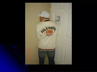
Lighting View Recognizing Faces?
Outline Bayesian Classification Principal Component Analysis (PCA) Fisher Linear Discriminant Analysis (LDA) Independent Component Analysis (ICA)
Bayesian Classification Classifier & Discriminant Function Discriminant Function for Gaussian Bayesian Learning and Estimation
The choice of D-function is not unique Classifier & Discriminant Function • Discriminant function gi(x) i=1,…,C • Classifier • Example • Decision boundary
Multivariate Gaussian x2 principal axes x1 • The principal axes (the direction) are given by the eigenvectors of ; • The length of the axes (the uncertainty) is given by the eigenvalues of
x1 x2 Mahalanobis Distance Mahalanobis distance is a normalized distance
y2 x2 y1 x1 Whitening • Whitening: • Find a linear transformation (rotation and scaling) such that the covariance becomes an identity matrix (i.e., the uncertainty for each component is the same) y=ATx p(y) ~ N(AT, ATA) p(x) ~ N(, )
Disc. Func. for Gaussian • Minimum-error-rate classifier
Case I: i = 2I constant Liner discriminant function Boundary:
j i Example • Assume p(i)=p(j) Let’s derive the decision boundary:
Case II: i= The decision boundary is still linear:
Case III: i= arbitrary The decision boundary is no longer linear, but hyperquadrics!
Bayesian Learning • Learning means “training” • i.e., estimating some unknowns from “training data” • WHY? • It is very difficult to specify these unknowns • Hopefully, these unknowns can be recovered from examples collected.
Maximum Likelihood Estimation • Collected examples D={x1,x2,…,xn} • Estimate unknown parameters in the sense that the data likelihood is maximized • Likelihood • Log Likelihood • ML estimation
generalize Case II: unknown and
Bayesian Estimation • Collected examples D={x1,x2,…,xn}, drawn independently from a fixed but unknown distribution p(x) • Bayesian learning is to use D to determine p(x|D), i.e., to learn a p.d.f. • p(x) is unknown, but has a parametric form with parameters ~ p() • Difference from ML: in Bayesian learning, is not a value, but a random variable and we need to recover the distribution of , rather than a single value.
Bayesian Estimation • This is obvious from the total probability rule, i.e., p(x|D) is a weighted average over all • If p( |D) peaks very sharply about some value *, then p(x|D) ~ p(x| *)
The Univariate Case • assume is the only unknown, p(x|)~N(, 2) • is a r.v., assuming a prior p() ~ N(0, 02), i.e., 0 is the best guess of , and 0 is the uncertainty of it. P(|D) is also a Gaussian for any # of training examples
n=30 p(|x1,…,xn) n=10 n=5 n=1 The Univariate Case The best guess for after observing n examples n measures the uncertainty of this guess after observing n examples p(|D) becomes more and more sharply peaked when observing more and more examples, i.e., the uncertainty decreases.
PCA and Eigenface Principal Component Analysis (PCA) Eigenface for Face Recognition
PCA: motivation • Pattern vectors are generally confined within some low-dimensional subspaces • Recall the basic idea of the Fourier transform • A signal is (de)composed of a linear combination of a set of basis signal with different frequencies.
x e xk m PCA: idea
PCA To maximize eTSe, we need to select max
Algorithm • Learning the principal components from {x1, x2, …, xn}
PCA for Face Recognition • Training data D={x1, …, xM} • Dimension (stacking the pixels together to make a vector of dimension N) • Preprocessing • cropping • normalization • These faces should lie in a “face” subspace • Questions: • What is the dimension of this subspace? • How to identify this subspace? • How to use it for recognition?
Eigenface The EigenFace approach: M. Turk and A. Pentland, 1992
An Issue • In general, N >> M • However, S, the covariance matrix, is NxN! • Difficulties: • S is ill-conditioned. Rank(S)<<N • The computation of the eigenvalue decomposition of S is expensive when N is large • Solution?
Solution I: • Let’s do eigenvalue decomposition on ATA, which is a MxM matrix • ATAv=v • AATAv= Av • To see is clearly! (AAT) (Av)= (Av) • i.e., if v is an eigenvector of ATA, then Av is the eigenvector of AAT corresponding to the same eigenvalue! • Note: of course, you need to normalize Av to make it a unit vector
Solution II: • You can simply use SVD (singular value decomposition) • A = [x1-m, …, xM-m] • A = UVT • A: NxM • U: NxM UTU=I • : MxM diagonal • V: MxM VTV=VVT=I
Fisher Linear Discrimination LDA PCA+LDA for Face Recognition
PCA When does PCA fail?
Linear Discriminant Analysis • Finding an optimal linear mapping W • Catches major difference between classes and discount irrelevant factors • In the mapped space, data are clustered
Solution I • If Sw is not singular • You can simply do eigenvalue decomposition on SW-1SB
Solution II • Noticing: • SBW is on the direction of m1-m2 (WHY?) • We are only concern about the direction of the projection, rather than the scale • We have
LDA PCA Comparing PCA and LDA
Lighting MDA for Face Recognition • PCA does not work well! (why?) • solution: PCA+MDA
Independent Component Analysis The cross-talk problem ICA
S1(t) x1(t) t t S2(t) x2(t) t t x3(t) t Cocktail party A Can you recover s1(t) and s2(t) from x1(t), x2(t) and x3(t)?
Formulation Both A and S are unknowns! Can you recover both A and S from X?
The Idea • y is a linear combination of {si} • Recall the central limit theory! • A sum of even two independent r.v. is more Gaussian than the original r.v. • So, ZTS should be more Gaussian than any of {si} • In other words, ZTS become least Gaussian when in fact equal to {si} • Amazed!
View Face Recognition: Challenges