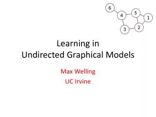
Learning in Undirected Graphical Models
Learning in Undirected Graphical Models. Max Welling UC Irvine. Overview. MRF Representation. Varieties of MRF: F ully observed, CRF, Hidden U nits. Relation to “Maximum Entropy”. Gradients, Hessian, Convexity. Gradient descend with exact gradients (low tree-width):

Learning in Undirected Graphical Models
E N D
Presentation Transcript
Learning in Undirected Graphical Models Max Welling UC Irvine
Overview • MRF Representation. • Varieties of MRF: • Fully observed, CRF, Hidden Units. • Relation to “Maximum Entropy”. • Gradients, Hessian, Convexity. • Gradient descend with exact gradients (low tree-width): • MRF, CRF, Hidden Units. • ML-BP and Pseudo-Moment Matching. • Alternative Objectives: • PL, Contrastive Free Energies, Contrastive Divergence, • Experiments • More methods: MCMC-MLE, Composite Likelihood, Persistent CD. • Herding • Max Margin Markov Networks • Structure Learning through L1-regularization • Bayesian Learning: • Langevin-CD, Laplace Approximation-BP (EP, MCMC). • Experiments • Conclusions
MRF Representation: Gibbs Distribution Assume a discrete sampling space X. Call Xk the group of variables in cluster “k”. Partition Function
Conditional Independencies • Consider a positive Gibbs distribution that factorizes as: • Consider a graphical representation G where all variables that reside inside a factor • are connected by an edge (a clique). • Consider the following conditional independence relationships (CIRs) for G: • if every path between X and Y is blocked by nodes in Z. • Then the CIRs for the graph G “correspond” to the CIRs in P. • -any P that factorizes over G satisfies these CIRs. • -if X and Y is not blocked by Z than there exists a P that factorizes over G in which • they are dependent given Z. Example CIR: Note: P could have a single factor f(1,2,5) or 3 factors f(1,2), f(1,5), f(2,5).
Examples Graphical representation of factorial CRF for the joint noun phrase chunking and part of-speech tagging problem, where the chain y represents the NP labels, and the chain w represents the POS labels Dynamic Conditional Random Fields: Factorized Probabilistic Models for Labeling and Segmenting Sequence Data. Charles Sutton, Andrew McCallum, KhashayarRohanimanesh. Journal of Machine Learning Research 8. 2007 Markov network model for super-resolution problem Example-based super-resolutionWilliam T. Freeman, Thouis R. Jones, and Egon C. Pasztor.
Maximum Entropy Jaynes (empirical distribution) Idea: We want to find a probability distribution P with moments . However, there are many such P’s. Find the one with the least “additional assumptions” = maximum entropy. Maximum entropy problem has the same solution as its dual: maximum likelihood problem. With: ; H(P) is the dual of log(Z), parameters play role of Lagrange multipliers.
Gradients & Hessian of L The log-likelihood of the data for the model P is given as: To optimize it we would need the first derivative: If we divide by “n” we see that the direction of steepest ascent is the difference between two averages: the average of the data and the average of the model. Hessian is given by: Since the Covariance is positive definite we conclude that L is concave! (this result only holds if there are no hidden variables).
Gradient Descent MRF Gradient descent: Looks simple, however: is intractable in MRF with high treewidth. We could approximate the gradient using approximate inference techniques. For instance we could use: 1) Loopy Belief Propagation. This is “fast” but may not converge as parameters get stronger. Also, the estimate of the gradients is biased at every iteration so we may end up far away from the true optimum. 2) MCMC. This is slow because we need to run a MCMC chain to convergence for every update. Also, if we don’t collect enough samples to average over we will have high variance in the estimates of the gradients. 3) Can we trade off bias and variance?
GD for CRF • Even for the gradients we need to perform inference separately for every data-case “i”. • However, the inference is only over the labels Y, not the feature space X. • Conditioning on evidence often makes the distribution peak at a small subset of states, • i.e. there are fewer modes in P(Y|x). • To learn good conditional models for Y|x we often need more data than for generative • models over Y,X. Our assumptions on P(X) regularize learning. • This reduces variance (and thus over-fitting) but may introduce bias.
GD for PO-MRF • Evaluating gradient involves inference over Z|x for every data-case PLUS one more time • on Z,X jointly without any evidence clamped. • Hessian is now no longer a covariance but a difference of covariances which can easily • get negative definite => L is no longer concave as a function of its parameters!
Pseudo-Moment Matching (1) • Simplest case: fully observed MRF. • Even in this case we need to estimate the intractable quantity • if we want to do gradient descent. • One idea is to approximate this expectation by running loopy belief propagation. • Wainwright argues that this is reasonable if both learning and testing use the same • approximate inference algorithm. • Unfortunately, as the parameters grow LBP is less likely to converge. • For the fully observed case, one can actually compute an analytical expression • for the final answer, called pseudo-moment matching. [Wainwright,Jaakkola,Willsky ’03]
Pseudo-Moment Matching (2) • Consider the following special case: • MRF is fully observed. • Features are state indicators for single variables and pairs of variables: • (one for every node and edge in G) • Then the Pseudo-Moment Matching solution is: • We are now guaranteed that at one of LBP fixed points we have: • Generalization to higher order indicator features and GBP exist. • Generalization to hidden units not clear. • Solution only uses local information while we know that Z couples all parameters.
Pseudo-Likelihood (1) Besag ‘75 • Instead of approximating the gradients we can also change the objective. • In the PL we replace: . • We maximize: • As , which we call “consistency”. • However, PL is less statistically efficient than ML. • This means that we would repeat the estimation procedure with n data-cases • many times, then the average will be correct (unbiased) but the variance will • larger than for ML. • Computationally, PL is much more efficient however because we only need to • normalize conditional distributions over a single variable. Computational Efficiency Statistical Efficiency
Pseudo-Likelihood (2) with: • Note that it is easy to compute these conditionals because the summation is over values • of only one variable. • Hessian is a little involved but negative definite, so the PL is a concave objective. • PL doesn’t work for partially observed MRFs. (Some parameters may diverge.) • Intuition: Think of every data-case as a sample. For each of them, relax one variable and let • it re-sample from . If the new samples so obtained are different than the • original samples, then you need to change the parameters. The model is not perfect yet.
Contrastive Free Energies • We relax the data-samples using some procedure. • If they systematically change the E[f], then the • parameters are imperfect and need to be updated. • For PL, we relax one variable at a time (one dimension) • and sum these contributions. • We can also relax by running a brief MCMC • procedure starting at every data-case. • Or we can relax a variational distribution Q on a • mean field free energy or the Bethe free energy. • Analogy (Hinton): • 1. I will tell you a story (data) • 2. You will explain it back to me (relax the data, mix) • 3. As soon as you make a mistake I will correct you • and you will have to start over again • (parameter update)
Contrastive Divergence (1) Hinton ‘02 REPEAT: Randomly select a mini-batch of data items of size n. Run n MCMC chains for r steps starting at the data items in the mini-batch. Compute feature expectations under the data distribution and the r-step samples: Update the parameters of the model according to*: Increase the number of steps r (this decreases bias). • Because we initialize the MCMC chains at the data-points (and not randomly) and we • run for only r steps we decrease the variance in the gradient estimate. • However, because we sample for only r steps we increase the bias. • As we increase r we trade less bias for more variance and computation. * This is not the gradient of the contrastive divergence:
Contrastive Divergence-RBM(2) • Restricted Boltzmann Machine (RBM) • has a layer of observed variables and a • layer of unobserved variables , • but no connections between them. • All variables are binary valued. • CD works well for this type of architecture because & • Update rule the same
Contrastive Divergence -Example (3) Osindero,et al‘05 J • Data: X: lowpass filtered greyscale images. • U=Z are hidden variables that model the • precision for the conditional Gaussian P(X|U) • Variables s=Jx are organized on a 2-d grid, and • W only connects to a small neighborhood of • s-variables. • x,u are continuous.
Some Experimental Results Parise, Welling ‘05 Binary values (Boltzmann machine) Fully observed Square grid of size 7x10. Parameters sampled from U[-0.1,0.1] Vary nr of data-cases sampled from model
Some Experimental Results Parise, Welling ‘05 Binary values (Boltzmann machine) Fully observed Square grid of size 7x10. Parameters sampled from U[-d/2,d/2], vary d N = 2000
Some Experimental Results Parise, Welling ‘05 Binary values (Boltzmann machine) Fully observed From 7x7 grid to complete graph by adding edges Weights sampled from U[-0.1,0.1] N = 10 x nr. parameters
Some Experimental Results Parise, Welling ‘05 Binary values (Boltzmann machine) Fully observed, 6x6 grid N = varies Real data, cropped 6x6 images from USPS digits (first learn parameters using PL, then sample data from it)
Some Experimental Results Parise, Welling ‘05 Binary values (Boltzmann machine) Fully observed From 6x6 grid to complete graph by adding edges N = 10 x nr. parameters Real data from USPS digits (first learn parameters using PL, then sample data from it)
Some Experimental Results Parise, Welling ‘05 Binary values (Restricted Boltzmann machine) 10 Hidden and 10 Visible nodes all connected OR 7x10 biparite grid (alternating visible hidden). All interactions +ve sampled from U[0,d], vary d N = 12000 (RBM), 20000 (Grid). Initialize learning at true value (local minima)
Some Experimental Results Parise, Welling ‘05 Binary values (Restricted Boltzmann machine) 10 Hidden and 10 Visible nodes all connected OR 7x10 biparite grid (alternating visible hidden). All interactions +ve sampled from U[0,0.1] Vary N Initialize learning at true parameter values (local minima)
Conclusions Experiments • Fully Observed: PMM only works if interactions strength is small and sparsity is high. • For FO problems, PL and CD worked equally well, but PL is faster. • For Partially observed problems PMM and PL don’t work, but CD works well. • For PO problems (CD), the bias and variance decreased as interaction strength increased. • Since variance decreases faster than bias, more parameters become • statistically significantly biased. • As N increases bias and variance decrease and the • number of statistically significantly biased parameters also • also decreases. If model is fully observed: use PL If model is partially observed: use CD
MCMC-MLE Geyer ‘91 • If we can easily sample from q(X), and q(X) is close to p(X) then this can be used • to approximate Z. • The gradient can be approximated as: • As we update parameters, the weights quickly • degenerate (effective sample size = 1). • One can resample from the weights, • and rejuvenate by running MCMC for some steps • to improve the health of the particle set: Particle Filtered MCMC [Asuncion et al, 2010] Importance weights:
Composite Likelihood Lindsey, ‘88 • We can easily generalize PL so that evaluate the probability at arbitrary blocks • conditioned on (different) arbitrary blocks. • This is called the composite likelihood: • We want that at least every variable appears in some bock Ac. • We want that for any particular component c, Ac and Bc are different. • We want that Ac is not empty for every c. • CL is still concave! • Gradient: • We can now interpolate between ML and PL.
Persistent CD Younes ‘89, Neal ‘92 Tieleman ‘08 • Instead of restarting the MCMC chains at the data-items, we can also • initialize them at the last sample before the parameters were updated. • This is exactly the same running Markov chains for some model P, and • regularly interrupting these chains to change P a little bit. • If the changes to P are small enough so that the chain can reach equilibrium • between the updates, then the chains will track the distribution P and • provide unbiased samples to compute the gradients. • Example of a Robbins-Monro method to find a solution of: • using a stochastic approximation method. • This implies that we need a decreasing sequence of step-sizes such that:
Herding Welling ‘09 • Take the zero temperature limit: • Then T*L0 converges to: • The gradient for some given state S is given as: • Where: • Herding iterates these steps. It does not try to • find the maximum (that’s at 0), but it will generate • pseudo-samples {St} that will satisfy the constraints: • This function is: • Concave • Piecewise linear • Non-positive • Scale free Tipi function:
Example in 2-D s=[1,1,2,5,2... Itinerary: s=1 s=6 s=2 s=5 s=3 s=4
Grid Neuron fires if input exceeds threshold Synapse depresses if pre- & postsynaptic neurons fire. Threshold depresses after neuron fires
Example Chen et al 2011 Classifier from local Image features: Classifier from boundary detection: Combine with Herding + Herding will generate samples such that the local probabilities are respected as much as possible (project on marginal polytope)
Convergence Translation: ChooseStsuchthat: Then: s=1 s=6 Equivalent to “Perceptron Cycling Theorem” (Minsky ’68) s=[1,1,2,5,2... s=2 Note: this implies that we do not have To solve the MAP problem at every iteration As long as the CPT holds! s=5 s=3 s=4
Period Doubling As we change R (T) the number of fixed points change. T=0: herding Logistic map: “edge of chaos”
Herding with Hidden Units: RBM inputation through maximization
A New Learning Rule RBM Hopfield net Runs without the data. Dreaming about digits
Max-Margin Markov Networks Taskar et al ‘02 • If we don’t care about the probabilities but we do care about making the right decision, • then there is a “max-margin” alternative to CRFs. • On the training data we require that the energy of the true label (given the attributes) • is lower than the energy of any other possible state , by pre-specified margin. • The margin depends on (Y,yi)so that almost correct states Y have a smaller margin. • Optimization looks daunting because of exponentially many constraints. • However, we can add the constraints one-by-one (constraint generation). Often, • you are done after you added a polynomial nr. of constraints. • To find which constraints to add, you run MAP-inference on the current QP problem • for every data-case. If MAP states satisfy constraints you are done.
Structure Learning: L1-regularization Lee et al ’06, Abbeel et al ‘06 • How can we decide which features to include in the model? • One practical way is to add L1-regularization to the parameters: • The L1 penalty will drive unimportant features to 0, effectively removing them from • the model. • We can thus iteratively add features to the model until the score no longer increases. • There is a PAC-style bound to guarantee that the solution is close to the best solution • (in a KL-sense).
Bayesian Methods • “Doubly intractable” because of partition function and Bayesian integration over • parameters. • Even MCMC would require one to compute Z for the old and proposed state at • every iteration. • A nifty algorithm exists that circumvents the computation of Z if we can draw • perfect samples from P(X). • We will discuss approximate MCMC & Laplace approximations. There is also an • approach for CRFs based on EP [Qi et al ’05]. • Without hidden units the posterior is unimodal. • With hidden units the problem is “triply intractable” because a very large • number of modes may appear in the posterior. [Moller et al ‘04, Murray et al. ‘06]
Bayesian Methods (1)Approximate Langevin Sampling [Murray, Ghahramani ’04] • MCMC with accept/reject requires the computation of Z for every sample drawn. • However, Langevin sampling does not requires this: • (catch: this only samples correctly when ) . • Idea: Let’s try for finite stepsizes. However, we still need the gradient. • Idea: Let’s use contrastive divergence gradients (brief MCMC chains started at the data). • This approximate sampling scheme worked well empirically. • (gradients based on mean field did not work, gradients based on BP sometimes worked).
Bayesian Methods: Laplace + BP Parise & Welling ’06, Welling & Parise ‘06 • Unlike MCMC, we only have to compute Z once at the MAP state. • We can approximate Z using “Annealed Importance Sampling” or the Bethe free energy. • C is the covariance between all fairs of features: • Approximate log(Z) with Bethe free energy, and C using “linear response propagation” • LRP is an additional propagation algorithm after BP has converged. • For Bolzmann machine there is an analytic expression available. • Similar expression for CRFs. [Welling, Teh ’03]
Experiments: Methods (1) BP-LR-ExactGrads: BP-LR but using exact gradient to find the MAP-value of the parameters. Laplace-Exact: Laplace approximation, but computing the MAP value exactly and computing the covariance “C” and the partition function “Z” exactly. Annealed Importance Sampling = “ground truth”: [Neal 2001]. MCMC approach to compute evidence. This requires the exact evaluation of the Z at every iteration.
Experiments: Methods (2) We will vary: d = edge strength N = sample size Nr. edges
Experiments: Results (1) Vary the number of edges in 5 node model. (d=0.5/4)
Experiments: Results (2) Same experiment, but we plot difference with AIS (d=0.5/4)