Generalized Maximum Entropy Estimation Techniques in Econometrics
130 likes | 264 Vues
This review outlines advancements in estimation procedures through Generalized Maximum Entropy (GME) methods as articulated by Golan, Judge, and Miller in their 1996 work. It highlights the mathematical underpinnings of entropy, including Shannon's formula, and provides practical examples such as the application to unfair dice. The paper further discusses the implications of cross-entropy and the interplay between data and prior information in modeling ill-posed problems. It discusses constraints and the use of Lagrange multipliers for efficient solutions in estimation tasks.

Generalized Maximum Entropy Estimation Techniques in Econometrics
E N D
Presentation Transcript
Section ARE213Entropy Econometrics Estimation Procedure by Golan, Judge and Miller, 1996May 2006 Hendrik Wolff
Short Review on MaxEntropy • 1948 Claude Shannon: Information Entropy: • H(p) = - j=1 pj ln pj • Example of Dice: • 6 Support Points zj: z1, z2,..., z6 • Maxp H(p) • s.t. 3.5 = j=1...6 pjzj • 1.0 = j=1 pj • Solution: pj=1/6: • I.e. Uniform distribution of the discrete PDF f(z) • How does f(z) look like, if we don‘t observe the theoretical mean of 3.5? EXCEL
Solution to the ME-Problem Maxp H(p) = Maxp [- j=1 pj ln pj | y = j=1...6 pjzj , 1.0 = j=1 pj] Lagrange: L = - j=1 pj ln pj +λ (y - Zp) + θ(1.0 - p´1) δL/δp = - lnp - 1- Z´ λ - θ = 0 δL/δ λ = y- Zp = 0 δL/δ θ = 1-p´1 = 0 --> pk = exp(-Zk´λ) / Ωk(λ) with Ω(λ) = Σi=1...6 exp(-Zk´λ) No analytical solution (parallels Logit) Newton worsk since H is globally concave
Normalized Entropy Measuring the Information Content: „Importance of the contribution of each piece of data in reducing uncertainty“ S(p) = (- m pm ln pm) / ln(M) S(p) = 0 : no Uncertainty in the System: pi=1, pj=0 S(p) = 1 : Perfect Uncertainty
p: Posterior Probability q: Reference Probability Short Review on Cross-Entropy... 1951 Kullback & Leibler: CE(p,q) = j=1pj ln(pj /qj) Example: Unfair Dice EXCEL Normalized CE S(p) = ( - m pm ln pm ) / ( m-qm ln(qm))
1996: Golan, Judge & Miller Solution to ill-posed Problems via „Generalized ME“ Max H(p,w) = - m pm ln pm Max H(p,w) = - mkpmkln pmk Max H(p,w) = - mk pmk ln pmk - jnwjn ln wjn Max H(p,w) = - mk pmk ln pmk - jtwjt ln wjt • s.t. y=Xβ+e • with β=Zp, i.e.βk = m pmkZmk • e=Vw β is reparameterized into Analogue Separation of e into IK= (IK IM´)p IT= (IT IJ´)w
y z2 z1 x 1996: Golan, Judge & Miller Solution to ill-posed Problems via „Generalized ME“ Max H(p,w) = - m pm ln pm Max H(p,w) = - mkpmkln pmk Max H(p,w) = - mk pmk ln pmk - jnwjn ln wjn Max H(p,w) = - mk pmk ln pmk - jtwjt ln wjt s.t. y=Xβ+e β=Zp, e=Vw et[-2,2] Example: y = β1 + β2x , Prior info: βk[0,1] ,
y z2 z1 x From GME to GCE... Max H(p,w) = - m pm ln pm Max H(p,w) = - mkpmkln pmk Max H(p,w) = - mk pmk ln pmk - jnwjn ln wjn Min GCE(p,w|q,u) = + mk pmk ln pmk/qmk + jtwjt ln wjt/u jt s.t. y=Xβ+e with β=Zp, e=Vw
Min GCE(p,w|q,u) = γp´ln(p/q) +(1-γ)w´ln(w/u) s.t. α=ΓZp+Vw IK= (IK IM´)p IT= (IT IJ´)w Generalized Cross Entropy Input information---> Model ---> Outpu tinformationen , Z, q Y, X , V, u The Objective is to combine Data information and prior information in an efficient way to solve ill-posed problems.
Solution of the GCE-Approach Lagrange: L (p,q,λ,θ,τ) = p´ln(p/q) + w´ln(w/u) + λ´[α - ΓZp + Vw] + θ´[IK - (IK IM´)p] + τ´[IT - (IT IJ´)w] p = q exp(Z´Γ´λ) {(IK IM IM ´) [q exp(Z´Γ´λ) }-1 w = u exp(V´λ) {(IT IJ IJ ´) [u exp(V´λ) }-1 ---> pkm=qkm exp(zkmΓ´λ) / Ωk(λ) , with Ωk(λ) = Σmqkm exp(zkmΓ´λ) No closed form solution, but problem globally convex !
Solution GCE: Globally Convex Positive definite diagonal matrix P : Dimension (KMKM) W: Dimension (TJTJ)
Examples Heteroskedastizity: Time Series: Autocorrelation, ARCH etc. Cross-Section & Time Series (Panel): Statistical Model Selection: SUR: Simultaneous Systems: Dynamische Systems: LDV (Multinomiale, Censored Regression, Tobit Models):