Summary 3
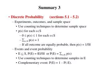
Summary 3. Discrete Probability (sections 5.1 - 5.2) Experiments, outcomes, and sample space Use counting techniques to determine sample space p(s) for each sS 0 p(s) 1 for each sS sS p(s) = 1 If all outcome are equally probable, then p(s) = 1/|S|

Summary 3
E N D
Presentation Transcript
Summary 3 • Discrete Probability (sections 5.1 - 5.2) • Experiments, outcomes, and sample space • Use counting techniques to determine sample space • p(s) for each sS • 0 p(s) 1 for each sS • sS p(s) = 1 • If all outcome are equally probable, then p(s) = 1/|S| • Events and event probability • E S, P(E) = |E|/|S| or P(E) = sE p(s) • Use counting techniques to determine samples in E • Complementary event: P(E) = 1 – P(-E).
Conditional probability P(E|F) • Definition: probability of E, given F (or in subspace F S) • Relation to joint probability • P(E|F) = P(EF)/P(F) or P(E|F) = |EF|/|F| • P(EF) = P(E|F)P(F) = P(F|E)P(E) • Inclusion-exclusion rule: P(EF) = P(E) + P(F) – P(EF) • Independence • Events E and F are independent of each other if P(E|F) = P(E) (E’s probability not depending on F) • P(EF) = P(E) + P(F) –P(E)P(F)
Bernoulli Trials • Experiment with two outcomes, s and f, • p = P(s), q = P(f) = 1– p (therefore p + q = 1) • n independent trials with k s (and n – k f) C(n, k)pkqn-k
Relations (sections 7.1 – 7.5) • Definitions. • (Binary) relation R from A to B: R AB: ordered pairs • Relation R on A: R AA • n-ary relation R A1A2…An • Functions are special cases of relations. • Properties of relations • Reflexive/irreflexive • Symmetric/asymmetric/antisymmetric • Transitive • Properties reflected in graph and matrix representations • Combining relations: R1 R2, R1 R2, R1 – R2, SR.
Equivalence relations • Definition: reflexive, symmetric and transitive. • Equivalence class: [a]R • For all b, if bRa, then b [a]R • aRb iff [a] = [b] iff [a] [b] • not aRb iff [a] [b] iff [a] [b] = • Partition of a set: (i) Ai for iI (ii) Ai Aj = , if i j (iii) iI Ai = S • All equivalence classes of R on A partition A.
Representing relations • Set of ordered pairs: • {(a, b)| aRb for all (a, b) AB} • 0 – 1 matrix • mij = 1, if (ai, bj)R, and • mij = 0, if (ai, bj)R. • Directed graph: (V, E) • V = A B ( or V = A if R is on A) • (a, b) E iff (a, b) R • Be able to convert between the three representations
Graphs (sections 8.1 – 8.4) • Definitions. • Simple, undirected and directed graphs. • Degree (indegree, outdegree) of vertex • Loop, isolated and pendant vertices • Special graphs Complete, cycle, bipartite, and complete bipartite, n-cube • Subgraph • Adjacency • For undirected graphs:vV deg(v) = 2|E| • For directed graphs: vV deg-(v) = vV deg+(v) = |E|
Representing graphs • Adjacency matrix • aij = 1 if {vi, vj} is an edge of G; and • aij = 0 otherwise. • Connectivity • Path, path length, simple path, circuit • A (undirected) graph is connected if there is a path between any pair of vertices • Strong and weak connected directed graphs • Connected components of a graph
Types of Questions • Conceptual • Definitions of terms • True/false • Simple questions • Problem solving • Work with small concrete example problems • Proofs • Simple theorems or propositions • Possible proof methods • Induction • Directed proof • Proof by contradiction

