Backpropagation Network in Artificial Neural Networks
120 likes | 271 Vues
This overview discusses the Backpropagation Network (BPN) as a popular type of Artificial Neural Network for classification and function approximation. It covers the structure, learning process, supervised learning, and gradient-descent techniques involved in training the network. The BPN aims to generalize and provide plausible outputs for unseen inputs by adjusting weights iteratively. By understanding its behavior post-training, one can utilize the network effectively.

Backpropagation Network in Artificial Neural Networks
E N D
Presentation Transcript
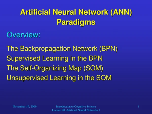
Overview: The Backpropagation Network (BPN) Supervised Learning in the BPN The Self-Organizing Map (SOM) Unsupervised Learning in the SOM Artificial Neural Network (ANN) Paradigms Introduction to Cognitive Science Lecture 20: Artificial Neural Networks I
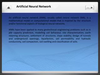
The Backpropagation Network • The backpropagation network (BPN) is the most popular type of ANN for applications such as classification or function approximation. • Like other networks using supervised learning, the BPN is not biologically plausible. • The structure of the network is as follows: • Three layers of neurons, • Only feedforward processing: input layer hidden layer output layer, • Sigmoid activation functions Introduction to Cognitive Science Lecture 20: Artificial Neural Networks I
synapses neuron i An Artificial Neuron o2 wi1 • o1 wi2 … oi … win on net input signal output signal Introduction to Cognitive Science Lecture 20: Artificial Neural Networks I
oi(t) = 0.1 1 = 1 0 neti(t) -1 1 Sigmoidal Neurons • The output (spike frequency) of every neuron is simulated as a value between 0 (no spikes) and 1 (maximum frequency). Introduction to Cognitive Science Lecture 20: Artificial Neural Networks I
The Backpropagation Network output vector o /desired output vector y • BPN structure: … O1 OK … H1 H2 H3 HJ … I1 I2 II input vector x Introduction to Cognitive Science Lecture 20: Artificial Neural Networks I
Supervised Learning in the BPN • In supervised learning, we train an ANN with a set of vector pairs, so-called exemplars. • Each pair (x, y) consists of an input vector x and a corresponding output vector y. • Whenever the network receives input x, we would like it to provide output y. • The exemplars thus describe the function that we want to “teach” our network. • Besides learning the exemplars, we would like our network to generalize, that is, give plausible output for inputs that the network had not been trained with. Introduction to Cognitive Science Lecture 20: Artificial Neural Networks I
Supervised Learning in the BPN • Before the learning process starts, all weights (synapses) in the network are initialized with pseudorandom numbers. • We also have to provide a set of training patterns (exemplars). They can be described as a set of ordered vector pairs {(x1, y1), (x2, y2), …, (xP, yP)}. • Then we can start the backpropagation learning algorithm. • This algorithm iteratively minimizes the network’s error by finding the gradient of the error surface in weight-space and adjusting the weights in the opposite direction (gradient-descent technique). Introduction to Cognitive Science Lecture 20: Artificial Neural Networks I
f(x) slope: f’(x0) x0 x1 = x0 - f’(x0) x Supervised Learning in the BPN • Gradient-descent example: Finding the absolute minimum of a one-dimensional error function f(x): Repeat this iteratively until for some xi, f’(xi) is sufficiently close to 0. Introduction to Cognitive Science Lecture 20: Artificial Neural Networks I
Supervised Learning in the BPN • Gradients of two-dimensional functions: The two-dimensional function in the left diagram is represented by contour lines in the right diagram, where arrows indicate the gradient of the function at different locations. Obviously, the gradient is always pointing in the direction of the steepest increase of the function. In order to find the function’s minimum, we should always move against the gradient. Introduction to Cognitive Science Lecture 20: Artificial Neural Networks I
Supervised Learning in the BPN • In the BPN, learning is performed as follows: • Randomly select a vector pair (xp, yp) from the training set and call it (x, y). • Use x as input to the BPN and successively compute the outputs of all neurons in the network (bottom-up) until you get the network output o. • Compute the error of the network, i.e., the difference between the desired output y and the actual output o. • Apply the backpropagation learning rule to update the weights in the network so that its output o for input x is closer to the desired output y. Introduction to Cognitive Science Lecture 20: Artificial Neural Networks I
Supervised Learning in the BPN • Repeat steps 1 to 4 for all vector pairs in the training set; this is called a training epoch. • Run as many epochs as required to reduce the network error E to fall below a threshold that you set beforehand. Introduction to Cognitive Science Lecture 20: Artificial Neural Networks I
Supervised Learning in the BPN • Now our BPN is ready to go! • If we choose the type and number of neurons in our network appropriately, after training the network should show the following behavior: • If we input any of the training vectors, the network should yield the expected output vector (with some margin of error). • If we input a vector that the network has never “seen” before, it should be able to generalize and yield a plausible output vector based on its knowledge about similar input vectors. Introduction to Cognitive Science Lecture 20: Artificial Neural Networks I